 |
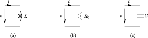
The equations relating voltage and current in the three one-ports, as well as their associated impedances are as follows:
| Inductor |
 |
(2.6) | ||||
| Resistor |
(2.7) | |||||
| Capacitor |
 |
(2.8) |
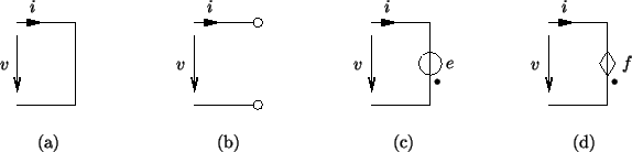
In addition to the one-ports mentioned above, we can also define the short-circuit, open-circuit, current source and voltage source (see Figure 2.4) by
| Short-circuit |
||||
| Open-circuit |
||||
| Voltage source |
||||
| Current source |
 |
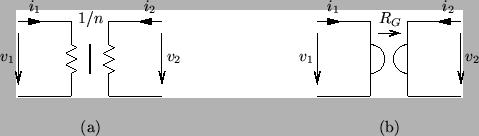
The two-ports which will occur most frequently in this thesis are the transformer and gyrator, both shown in Figure 2.5. Each of these two-ports has two voltage/current pairs, one for each port. The transformer has associated with it one free parameter ![]() , called the turns ratio, and the gyrator is defined with respect to a parameter
, called the turns ratio, and the gyrator is defined with respect to a parameter ![]() , as well as a direction, represented graphically by an arrow. The relation among the port variables in each case is given by
, as well as a direction, represented graphically by an arrow. The relation among the port variables in each case is given by
It is easily checked that both the transformer and gyrator are lossless two-ports. The gyrator is the first example we have seen so far of a non-reciprocal element--that is, its impedance matrix is not Hermitian; while we will not make nearly as much use of it here as the other elements, it will find a place in certain parts of this work, especially in dealing with physical systems which have a certain type of asymmetric coupling (see Chapter 5), in optimizing certain wave digital structures for simulation (see §3.12), and will play a pivotal role in linking digital waveguide networks to wave digital networks (see §4.10).
 |
There are other ![]() -ports of interest in network theory, many of which have been applied successfully in wave digital filter designs, such as circulators as well as time-varying [178] and non-linear elements [36,39,64,151], which have been used to study the propagation of nonlinear waves in lumped circuits [126]. For numerical integration purposes, however, the above set of elements proves to be an amply sufficient set of basic tools. An exception will be the non-linear distributed elements which appear in the circuit-based approach to fluid-dynamical problems; we mention these elements briefly in Appendix B.
-ports of interest in network theory, many of which have been applied successfully in wave digital filter designs, such as circulators as well as time-varying [178] and non-linear elements [36,39,64,151], which have been used to study the propagation of nonlinear waves in lumped circuits [126]. For numerical integration purposes, however, the above set of elements proves to be an amply sufficient set of basic tools. An exception will be the non-linear distributed elements which appear in the circuit-based approach to fluid-dynamical problems; we mention these elements briefly in Appendix B.