The Unit Element

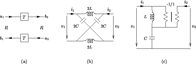
One wave digital two-port, called the unit element, is usually defined in the discrete-time domain, without reference to an analog counterpart; this wave digital two-port is shown in Figure 2.11(a). It was considered by Fettweis to be the ``most important two-port element'' [46], and was used extensively for realizability reasons in early wave digital filter designs, especially before the appearance of reflection-free ports [57]. It behaves exactly like a transmission line, and is in fact identical to the waveguide or bidirectional delay line which is the key component of the digital waveguide network [166], as we saw in §1.1.2. The unit element is time-invariant, and obviously lossless, though it is reactive (able to store energy).

Figure 2.11: The unit element and its continuous-time counterparts-- (a) a unit element, with port resistances $R$ and delays $T$, (b) its analog lattice form and (c) Jaumann form reference two-ports, with $L=\frac{RT}{4}$ and $C = \frac{T}{R}$.

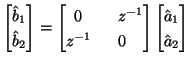
It should be clear, however, that we may simply apply the bilinear transform backwards in order to obtain a representation in the continuous time domain. The scattering relation for the unit element is

$$\begin{bmatrix}\hat{b}_{1}\\ \hat{b}_{2}\\ \end{bmatrix}= \begin{... ...\!\!&0\\ \end{bmatrix} \begin{bmatrix}\hat{a}_{1}\\ \hat{a}_{2}\\ \end{bmatrix}$$

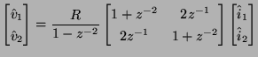
and transforming from wave variables back to voltages and currents via (2.14) gives

$$\begin{bmatrix}\hat{v}_{1}\\ \hat{v}_{2}\\ \end{bmatrix}= \frac{R... ...z^{-2}\\ \end{bmatrix} \begin{bmatrix}\hat{i}_{1}\\ \hat{i}_{2}\\ \end{bmatrix}$$

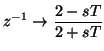
where $R$ is the port resistance at either port. The bilinear transform (2.11) may be inverted by

$$z^{-1}\rightarrow \frac{2-sT}{2+sT}$$

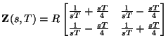
and we obtain, finally, a relationship between the continuous-time steady-state voltages and currents, with an impedance matrix (dependent on the time step $T$, assumed constant) given by

$${\bf Z}(s,T) = R\begin{bmatrix}\frac{1}{sT}+\frac{sT}{4}&\frac{1}... ...ac{sT}{4}\\ \frac{1}{sT}-\frac{sT}{4}&\frac{1}{sT}+\frac{sT}{4}\\ \end{bmatrix}$$

This defining equation for a two-port may be written as a lattice [55] (or Jaumann [132] equivalent) connection of an inductor and capacitor, each of whose values is now dependent on the choice of the time step, $T$. See Figures 2.11(b) and (c).

We mention this representation because in the distributed case, it will be possible to define multidimensional unit elements which will be very helpful in integrating digital waveguide networks (see Chapter 4) into the multidimensional wave digital filter framework (see Chapter 3). The necessary manipulations, which are quite similar to the ones performed above, are carried out in §4.10.