Discretization in the Spectral Domain

If our network or $N$-port is linear and shift-invariant, it is also possible to view the discretization procedure as a spectral mapping, just as in the last chapter. Consider now the case where the problem domain is some $n$-dimensional space, with coordinates $\mathbf{u}=[x_{1},\hdots,x_{n},t]^{T}$, and where we have changed coordinates to $\mathbf{t}=[t_{1},\hdots, t_{k}]^{T}$, with $k\geq n+1$ via a transformation of type (3.21). The defining equation of an MD inductor of direction $t_{j}$ for any $j=1,\hdots,k$ is

$$v = L\frac{\partial i}{\partial t_{j}}$$

and for an exponential state at frequencies ${\bf s_{t}}$, we have

$$\hat{v}=Ls_{j}\hat{i}$$

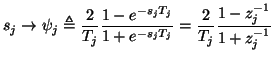
where $v=\hat{v}e^{{\bf s_{t}}^{T}{\bf t}}$ and $i=\hat{i}e^{{\bf s_{t}}^{T}{\bf t}}$. The ``impedance'' is here $Z = Ls_{j}$ and clearly satisfies MD positive realness criterion given in (3.31) (and furthermore is MD-lossless) if $L\geq 0$ . As in the lumped case, the trapezoid rule, now applied in the $t_{j}$ direction, can be interpreted as a spectral mapping

$$s_{j}\rightarrow \psi_{j} \triangleq \frac{2}{T_{j}}\frac{1-e^{-s_{j}T_{j}}}{1+e^{-s_{j}T_{j}}}= \frac{2}{T_{j}}\frac{1-z_{j}^{-1}}{1+z_{j}^{-1}}$$ (3.42)

where $T_{j}$ is some arbitrary step-size in the $t_{j}$ direction. For notational purposes, we have used

$$z_{j}^{-1} = e^{-s_{j}T_{j}}$$

to represent the frequency domain equivalent of a unit shift in the $t_{j}$ direction. In complete analogy with the lumped case, (3.43) implies that

$${\rm Re}(s_{j})\gtreqqless 0\hspace{0.2in} \Longleftrightarrow\hs... ...0\hspace{0.2in} \Longleftrightarrow\hspace{0.2in} \vert z_{j}\vert\gtreqqless 1$$

This shift can of course also be written in terms of delays and shifts in the $\mathbf{u}$ coordinates. For example, consider the coordinate transformation defined in (3.18). In this case we have, in the frequency domain,

$$s_{1} = \frac{1}{\sqrt{2}v_{0}}s_{t}+\frac{1}{\sqrt{2}}s_{x}\notag$$

$$s_{2} = \frac{1}{\sqrt{2}v_{0}}s_{t}-\frac{1}{\sqrt{2}}s_{x}\notag$$

where $s_{t}$ and $s_{x}$ are the frequency variables conjugate to $t$ and $x$ respectively. (We assume that our spatial domain is of infinite extent, so that $s_{x}$ corresponds to an imaginary Fourier transform variable.) Suppose we have also chosen the step-sizes in the two coordinates such that the grids overlap, that is, $T_{1}=\sqrt{2}\Delta=\sqrt{2}v_{0}T$, where $T$ is the shift in the pure time direction. Then, for a shift of $T_{1}$ in the $t_{1}$ direction, we can write

$$e^{-s_{1}T_{1}}=e^{-\frac{1}{\sqrt{2}v_{0}}s_{t}T_{1}-\frac{1}{\sqrt{2}}s_{x}T_{1}} = e^{-s_{t}T-s_{x}\Delta}$$

or

$$z_{1}^{-1}=z^{-1}w^{-1}$$ (3.43)

where $z^{-1}$ represents a delay of duration $T$ in the time direction, and $w^{-1}$ corresponds to a shift over distance $\Delta$ in the positive space direction. Similarly, we can write

$$z_{2}^{-1}=z^{-1}w$$ (3.44)

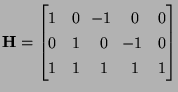
For a more complex example, consider again the transformation defined by

$$\mathbf{H} = \begin{bmatrix}1&0&\!\!-1&0&0\\ 0&1&0&\!\!-1&0\\ 1&1&1&1&1 \end{bmatrix}$$

which maps coordinates $[x,y,t]^{T}$ to a five-dimensional coordinates $[t_{1},t_{2},t_{3},t_{4},t_{5}]^{T}$. A shift of $T_{1} = \Delta$ in direction $t_{1}$ corresponds to a transmittance of the form

$$z_{1}^{-1} = e^{-s_{1}T_{1}} = e^{-(s_{x}+\frac{1}{v_{0}}s_{t})\Delta} = e^{-(s_{x}\Delta+s_{t}T)} = z^{-1}w_{x}^{-1}$$

where $w_{x}$ represents a unit shift (of length $\Delta$) in the $x$-direction, and as before, $z^{-1}$ corresponds to a unit delay of $T = \Delta/v_{0}$. The other shifts can be written as

$$z_{2}^{-1}=z^{-1}w_{y}^{-1} \hspace{0.2in} z_{3}^{-1}=z^{-1}w_{x} \hspace{0.2in} z_{4}^{-1}=z^{-1}w_{y} \hspace{0.2in} z_{5}^{-1}=z^{-1}$$

where $w_{y}$ represents a unit shift (of length $\Delta$) in the $y$ direction. At a given grid point in the old coordinates, the unit delays $z_{1}^{-1},\hdots, z_{4}^{-1}$, interpreted as directional shifts, refer to points on the grid at the previous time step, and located one grid point away in the $-x$, $-y$, $x$ and $y$ directions, respectively. The unit delay $z_{5}^{-1}$ is simply a unit time delay.

It is important to note the manner in which the special character of the coordinate transformation manifests itself here. Due to the positivity requirement on the elements of the last column of $\mathbf{H}$, a unit delay in any of the directions $t_{j}$ will always include some delay in the pure time direction. By means of this requirement, and the introduction of wave variables, MDWD networks can, in the same way as their lumped counterparts, be designed in which delay-free loops do not appear. Such networks, when used for simulation, will give rise, in general, to explicit numerical schemes [176].