Boundary Termination of the Mindlin Plate

There are four common types of conditions applied at a plate boundary [94]. At a southern boundary, parallel to the $x$ axis, the four conditions can be written as

These conditions are again lossless, and of the form of (3.8). (We note that conditions on $v$, $\omega_{x}$ and $\omega_{y}$ in (5.44) are usually written in terms of their time integrals $w$, $\psi_{x}$ and $\psi_{y}$, but the formulation above is equivalent.) The same conditions also reduce to a similar set of conditions which can be applied to the classical plate, as defined by [17].

As we mentioned in §5.2.4, the passive boundary termination of an MDWD network, such as that shown in Figure 5.16, is not at all straightforward. Indeed, it is somewhat complicated by the fact that we must approximate all the system variables at any given grid point on the boundary, and we were not able to implement a stable termination for this network. The ``wave-canceling'' method [107] discussed in §3.11 becomes exceedingly complex when vector wave variables and reflection-free ports are involved; passivity is not easy to ensure.

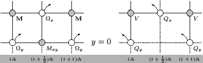
Termination of the DWN derived from the MDKC of Figure 5.17, operating on the computational grid of Figure 5.18, however, is simpler, because we are able to work directly with the termination of the lumped mesh representation. Suppose we choose our southern boundary at $y=0$ according to Figure 5.19. The only quantities to be calculated in this arrangement will be $Q_{y}$ and $\Omega_{y}$, at coincident series scattering junctions, and $M_{xy}$ at parallel scattering junctions. This arrangement is to be preferred, because we do not need to worry about the termination of the vector scattering junctions at which ${\bf M} = [M_{x}, M_{y}]$ is calculated.

Figure: Southern computational grid boundary at $y=0$ for the DWN for Mindlin's system.

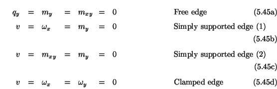
The southern boundary terminations corresponding to the four conditions (5.44) are shown in Figure 5.20. The conditions $q_{y} = 0$ and $\omega_{y} = 0$ that appear in (5.44a) and (5.44d) can be dealt with rather simply, by terminating the boundary series junctions at which the junction currents $Q_{yJ}$ and $\Omega_{yJ}$ are calculated in an open circuit. For these conditions, the gyrator coupling between the two subnetworks (indicated by curved arrows in Figure 5.19) may be dropped entirely. Similarly, the condition $m_{xy} = 0$ can be implemented by short-circuiting the appropriate parallel boundary junctions.

The other conditions, involving variables not calculated directly on the boundary require a slightly more involved treatment; the analysis is similar to that performed in §4.4.4, and the termination problem becomes (for the most part) that of setting the self-loop immittances at the boundary junctions which can not be trivially terminated in an open or short circuit. To this end, we provide the waveguide immittances at the junctions in the problem interior at which $M_{xyJ}$, $\Omega_{yJ}$ and $Q_{yJ}$ are calculated. From Figure 5.17, it is possible to read off these values directly. As for the DWN for the Timoshenko system in §5.2.2, immittances in the two overlapped networks are distinguished by a tilde ( $\tilde{\hspace{0.1in}}$). For example, at a parallel junction in the five-variable grid at location $x=(i+\frac{1}{2})\Delta$, $y=j\Delta$, for $i$ and $j$ integer, where we calculate $M_{xyJ,i+\frac{1}{2},j}$ (see Figure 5.18), there are waveguide connections to the north, south, east and west; their admittances are defined as

$$\tilde{Y}_{y^{+},i+\frac{1}{2},j}= \tilde{Y}_{y^{-},i+\frac{1}{2}... ...}{2},j}= \tilde{Y}_{x^{-},i+\frac{1}{2},j} = \frac{1}{R_{15}} = \frac{1}{r_{3}}$$

respectively, which are simply the admittances of the multidimensional unit elements from Figure 5.17. Similarly, the four connecting waveguide impedances at series junctions at locations $x=i\Delta$, $j=i\Delta$ (at which $\Omega_{yJ,i,j}$ are calculated) will have impedances

$$\tilde{Z}_{y^{+},i,j} = \tilde{Z}_{y^{-},i,j} = R_{14} = r_{2}\hspace{0.5in}\tilde{Z}_{x^{+},i,j} = \tilde{Z}_{x^{-},i,j} = R_{15} = r_{3}$$

In the other waveguide mesh (on the right in Figure 5.18), the connecting northward and southward impedances at the series junctions at which $Q_{yJ,i,j}$ is calculated will be

$$Z_{y^{+},i,j} = Z_{y^{-},i,j} = R_{9} = r_{1}$$

The self-loop immittances at the three types of junctions will be

$$\begin{eqnarray}\tilde{Y}_{c,i+\frac{1}{2},j} &=& \frac{1}{R_{8}}... ...Z_{c,i,j} &=& R_{2} = \frac{2v_{0}}{(\kappa^{2}Gh)_{i,j}}-2r_{1} \end{eqnarray}$$ (5.47a)

We assume $r_{1}$, $r_{2}$ and $r_{3}$ to be chosen according to (5.37), (5.40) and (5.41) respectively.