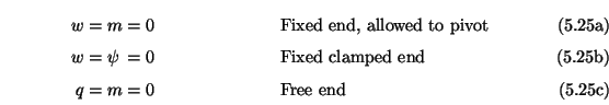
There are several possibilities for the implementation of these boundary conditions (5.25) at a boundary grid point in the MDWD network or any of the mentioned DWN structures. Through simulation, we have determined that the use of reflection-canceling waves at the boundary, as per the method of [107], does not lead to a passive termination. This statement also holds for the termination of the plate and shell models that we will discuss shortly; violent instabilities may appear in these systems, even though the termination of the simpler transmission line and parallel-plate networks by this method is not problematic. At present, the termination of a MDWD network is very poorly understood, even by experts [115]. Indeed, as we mentioned in §3.11, there is not, as yet, a general theory of boundary termination of MDWD networks [142]. We refer to §6.2.3 for a discussion of a possible avenue of approach.
For this reason, we decided to retreat from this problem, and work with the termination of the DWN, in its conventional lumped form. When a network is viewed in this way, it is much simpler to see how boundary conditions may be set such that passivity may be maintained. The difficulty in working with the expanded signal flow diagram for a MDWD network is that unlike the DWN, there is no port structure in this case; in the DWN, applying lumped terminations to junctions on the boundary is straightforward.
Because we looked at the termination of the (1+1)D transmission line, (2+1)D parallel-plate and Euler-Bernoulli systems in this way in §4.3.9, §4.4.4 and §5.1.3 respectively, we simply present the terminations corresponding to boundary conditions (5.25). We have chosen here to work with the DWN shown in Figure 5.9, although the termination of the networks of Figures 5.10 and 5.11 is equally simple. In addition, we align the parallel junctions (at which ![]() and
and ![]() are calculated) with the left end point (say) of the beam, located at
are calculated) with the left end point (say) of the beam, located at ![]() . In this way, we avoid the slight additional complication of the coupling that occurs if the series junctions are placed at the boundary (though we will be forced to face this issue when we set boundary conditions in the Mindlin plate network in §5.4.2). The three terminations are shown in Figure 5.12.
. In this way, we avoid the slight additional complication of the coupling that occurs if the series junctions are placed at the boundary (though we will be forced to face this issue when we set boundary conditions in the Mindlin plate network in §5.4.2). The three terminations are shown in Figure 5.12.
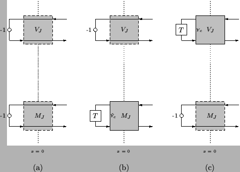 |
A condition ![]() (implying
(implying ![]() ) or
) or ![]() is easily implemented by short-circuiting the appropriate junction. For the condition
is easily implemented by short-circuiting the appropriate junction. For the condition ![]() , it is easy to show that we should choose the self-loop admittance to be
, it is easy to show that we should choose the self-loop admittance to be
![]() at the terminating junction at which
at the terminating junction at which ![]() is calculated. Similarly, for the condition
is calculated. Similarly, for the condition ![]() , we should choose
, we should choose
![]() at the junction at which
at the junction at which ![]() is calculated.
is calculated.