Next: Multi-grid Methods Using MDKCs
Up: Future Directions
Previous: Higher-order Accuracy
MDKC Modeling of Boundaries
One of the big hurdles yet to be overcome in the MDWD simulation method is the implementation of boundary conditions. As we mentioned briefly in §3.11, this is a very tricky business, and the approaches in the literature for simple model problems do not generalize to more complex systems. Setting boundary conditions for systems such as beams and plates was a time-consuming, and ultimately fruitless venture. We were forced to turn to DWNs, for which appropriate boundary conditions are much easier to find, because the DWN can be interpreted as a lumped network. The problem is that there is not, as yet, a general theory of boundary conditions for MDWD simulation methods [142]. In this section, we briefly mention a possible foundation for such a theory which is based on the ideas presented initially in [48,85,131] and outlined in §3.4.
Suppose that the problem of interest is  D, and defined with respect to coordinates
![$ {\bf u} = [x_{1},\hdots,x_{n},t]^{T}$](img2685.png) , or equivalently, to
, or equivalently, to  transformed coordinates
![$ {\bf t} = [t_{1},\hdots, t_{k}]^{T}$](img602.png) , with
, with  . We will assume that the problem has one spatial boundary, namely the hyperplane
  , and is defined over a time interval
 ![$ [0,t_{f}]$](img2687.png) . As such, the problem domain
. As such, the problem domain  is then
or its equivalent in the  coordinates, obtained under a transformation of the form (3.21).
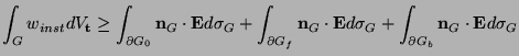
We restate the energy balance for an
coordinates, obtained under a transformation of the form (3.21).
We restate the energy balance for an  -port defined over , which is
where  is the instantaneous applied power at the ports,
  is an internal source power,
  is dissipated power, and
  is a column -vector representing stored energy flux;
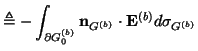
 is the differential volume element. As mentioned previously, the -port is integrally MD-passive over if
 |
(6.3) |
for some , all of whose components in the coordinates are positive everywhere in . Here,
 is the boundary of ,
 is the unit outward normal, and
 is a differential surface element on the boundary.
Note that
consists of the union of three sets of points, i.e.,
where, in terms of the physical  coordinates
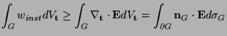
We can thus rewrite (6.3) as
For a closed network--that is, an -port with no free terminals (corresponding to a complete system of PDEs)--the instantaneous applied power is zero, so we are left with
 |
(6.4) |
In other words, the stored power flux leaving the boundary must be negative (the -port is passive).
Suppose, now, that there is an  D -port defined on the spatial boundary
 of . Renaming this region
  , we have another energy balance
over coordinates
 derived from physical coordinates
![$ {\bf u} = [x_{2},\hdots,x_{n},t]^{T}$](img2710.png) on . The quantities
on . The quantities
 ,
,
 ,
,
 and
and
 are the applied power, source power, dissipated power, and stored energy flux in the boundary network. Again, if the boundary network is passive, we have
 |
(6.5) |
where
 is the boundary of the region , and consists of the union of the two regions
so that we have, finally,
 |
(6.6) |
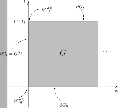
The boundary network is intended to model a passive distributed termination to the problem defined over the region . It should be clear that if both networks are passive, then if the transfer of energy between them is passive, then the terminated system as a whole will be passive. See Figure 6.3 for a representation of the relevant regions.
Figure 6.3:
A region with one spatial boundary.
 |
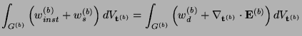
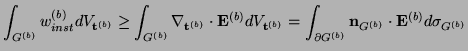
We can ensure this by requiring that the power applied through the ports of the boundary network over the region is equal to the stored energy flux of the interior network leaving through its spatial boundary (recall that we have set
 ). In other words, we require
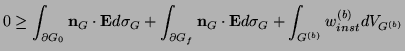
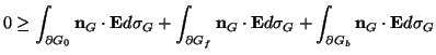
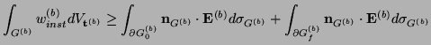
Inequality (6.4) can then be rewritten as
or, by employing (6.6), as
 |
(6.7) |
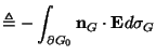
From (3.30), the quantities in (6.7) have the following interpretation:
The negative signs in the definitions of the initial energies result from the fact that the outward normal to
 and
and
 points in the negative time direction. As such, (6.7) can be restated simply as
or, in other words: the total energy stored in the interior and boundary networks must not increase as time progresses.
It is straightforward to extend this idea to more complex boundaries. For example, if the region were to be defined by
so that there is a corner at
 , we could model passive boundary conditions using four networks: an D network for the interior of , two D networks for the two ``faces,'' and a
  D network for the corner itself; an energy inequality similar to (6.7) results.
Here, we have said absolutely nothing about discretization (and indeed, we have not investigated this problem in any detail). We have, however, indicated the possibility for arbitrary distributed passive boundary termination of a given MDKC; only lumped conditions have been examined so far in the literature.
Next: Multi-grid Methods Using MDKCs
Up: Future Directions
Previous: Higher-order Accuracy
Stefan Bilbao
2002-01-22