Other Waveguide Networks for Timoshenko's System

For completeness sake, we mention two other DWNs for the Timoshenko system for which there is no need for the coupling reflection-free ports; all junctions are isolated from one another by delays. They were derived separately, and not through the manipulation of an MDKC. In fact, they can be arrived at in this manner, but we will present only the resulting structures. We mention them primarily because although they are quite similar to the DWN of the last section, the passivity condition on the immittance values leads to a radically different bound on $v_{0}$, the space step/time step ratio.

The difference between the two forms presented here is only in the coupling between the two lines, each type of which gives rise to a different type of offset sampling. For example, in the configuration shown in Figure 5.10, we calculate $Q_{J}$ and $M_{J}$ at the same time instant, and at the same grid location, whereas in Figure 5.11, the updating of $Q_{J}$ with respect to $M_{J}$ is staggered in both time and space.

Figure 5.10: An alternate DWN for Timoshenko's system.

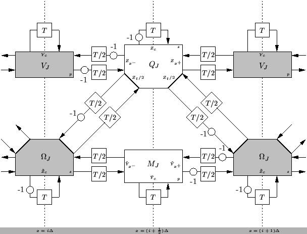Figure 5.11: Another alternate DWN for Timoshenko's system.

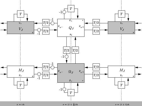There are many ways of setting the network immittances so as to approximate the Timoshenko system. Since both networks are simply just pairs of coupled (1+1)D transmission lines, the derivation of the constraints on the junction immittances is familiar. Because the two networks are so similar, we will state these constraints only for the network shown in Figure 5.11:

$$Z_{J,i+\frac{1}{2}} = \frac{2v_{0}}{(\overline{AG\kappa})_{i+\fra... ...e{\rho A})_{i}\hspace{0.2in}\tilde{Y}_{J,i} =\frac{2v_{0}}{(\overline{EI})_{i}}$$

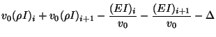
We use the bar notation again to indicate an approximation to at least second-order accuracy in the spatial step $\Delta$, and the tilde to distinguish between the immittances in the two transmission lines. Before we begin setting the immittances values, however, we must comment on the coupling waveguides which run between the parallel junctions which calculate $Q_{J}$ and $\Omega_{J}$; each such waveguide has a non-reciprocal character (as evidenced by the sign inversion in only one of the two signal paths). We have left the admittance of this coupling waveguide independent of position. The reason for this is seen from the difference equations in the junction variables. For example, in the configuration of Figure 5.11, we have, after following through familiar manipulations,

$$Q_{J,i+\frac{1}{2}}(n+{\textstyle \frac{1}{2}}) = Q_{J,i+\frac{1}... ...ac{1}{2}}}\left(V_{J,i+1}(n)-V_{J,i}(n)-Z_{t}\Omega_{J,i+\frac{1}{2}}(n)\right)$$

which will approximate (5.17b) only if $Z_{t}=\Delta$. The same statement is true of the other configuration as well (where the admittance of each coupling waveguide is set to $Z_{t}/2$).

It is convenient to set the immittances such that the self-loops at the parallel junctions (recall the transmission line) can be dropped entirely from the calculation; in fact, in this lossless case, we can drop the explicit calculation of $V_{J}$ and $M_{J}$ altogether if we wish, since when the self-loops at these junctions disappear, we are left with simple ``through'' junctions which do not scatter (recall Figure 4.14). Eventually, though, we may wish to have access to this variable because it is indeed the time derivative of $w$, the primary dependent variable of interest. We thus set

$$Z_{x^{-},i+\frac{1}{2}} = Z_{x^{+},i-\frac{1}{2}} = \frac{1}{v_{0... ...{v_{0}}\hspace{0.3in}Z_{t,i+\frac{1}{2}} = \tilde{Z}_{t,i+\frac{1}{2}} = \Delta$$

and

$$Z_{c,i+\frac{1}{2}} = \frac{v_{0}}{(AG\kappa)_{i}}+\frac{v_{0}}{(AG\kappa)_{i+1}}-\frac{1}{v_{0}\rho_{i}A_{i}}-\frac{1}{v_{0}\rho_{i+1}A_{i+1}}-\Delta$$

$$\tilde{Z}_{c,i+\frac{1}{2}} = v_{0}(\rho I)_{i} + v_{0}(\rho I)_{i+1}-\frac{(EI)_{i}}{v_{0}}-\frac{(EI)_{i+1}}{v_{0}}-\Delta$$

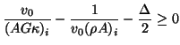
It is quite interesting to examine the positivity conditions on the self-loop admittances. For example, $Z_{c,i+\frac{1}{2}}$ will be positive if, for all integer $i$, we have

$$\frac{v_{0}}{(AG\kappa)_{i}}-\frac{1}{v_{0}(\rho A)_{i}}-\frac{\Delta}{2}\geq 0$$

which, using $v_{0} = \Delta/T$, is equivalent to

$$\Delta^{2}\left(\frac{1}{(AG\kappa)_{i}}-\frac{T}{2}\right) \geq \frac{T^{2}}{(\rho A)_{i}}$$

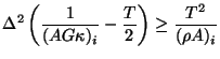
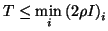
It is easy to see that, in contrast to the stability conditions we derived for the various transmission lines, for the ideal beam, and for Timoshenko's system in §5.2.1, for a passive realization there is now a maximum time step for the scheme regardless of the spatial step. That is, the above condition can be true only when

$$T\leq \min_{i}\frac{2}{(AG\kappa)_{i}}$$

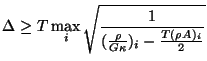
Assuming that this condition is met, we then must have

$$\Delta \geq T\max_{i}\sqrt{\frac{1}{(\frac{\rho}{G\kappa})_{i}-\frac{T(\rho A)_{i}}{2}}}$$

A positivity requirement on $\tilde{Z}_{c,i}$ yields a similar set of conditions,

$$T \leq \min_{i}\left(2\rho I\right)_{i} \hspace{0.2in}\Delta \geq T\max_{i}\sqrt{\frac{(EI)_{i}}{(\rho I)_{i} - \frac{T}{2}}}$$

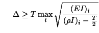In the limit as $T$ becomes small, both conditions on the spatial step size $\Delta$ approach conventional CFL-type bounds (recall the wave speeds implied by Timoshenko's system, mentioned in the beginning of this section); both must be satisfied for the waveguide network to be concretely passive, though they may be stable in the Von Neumann sense (see Appendix A). It would appear that the special character of these passivity conditions on the scheme are the direct result of the approximation of the memoryless asymmetric line coupling by a reactive waveguide coupling.