


Next: Improved MDKC for Timoshenko's
Up: Timoshenko's Beam Equations
Previous: Boundary Conditions in the
Simulation: Timoshenko's System for Beams of Uniform and Varying Cross-sectional Areas
We present here some two simple DWN simulations of the Timoshenko beam equations. In both cases, we have made use of the DWN of Figure 5.9, which was derived directly from an MDKC (shown in Figure 5.7). We simulate the behavior of a square prismatic steel beam, of length  m, under the application of an initial transverse velocity distribution at the beam center which has the form of one period of a raised cosine, of wavelength 5cm and amplitude 0.0005 m/s. In the first simulation, the beam is assumed to have a uniform thickness of 2 cm, and the boundary conditions are of the free type at either end; the evolution of the velocity distribution is shown in Figure 5.13. In the second simulation, the beam is assumed to be of linearly-varying thickness, from 1 cm at the left end to 3 cm at the right end. The area
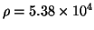
  thus varies quadratically, and the moment of inertia quartically. In this second case (shown in Figure 5.14), the boundary conditions are assumed clamped. The material parameters for steel are taken to be
 kg/m
kg/m ,
,
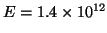 N/m
N/m ,
,
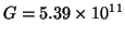 N/m, and Timoshenko's coefficient for a beam of square cross-section is
 [83]. In both simulations, we operate using a grid spacing of
  m, and the time step is chosen to be at the passivity limit. From (5.24), and given the above values of the material parameters of the beam,
  is chosen to be 5.1
 m/s for the uniform beam, and 4.59
 m/s for the beam of varying thickness.
Figure 5.13:
Simulation: evolution of the transverse velocity distribution along a Timoshenko beam of uniform thickness, with free ends.
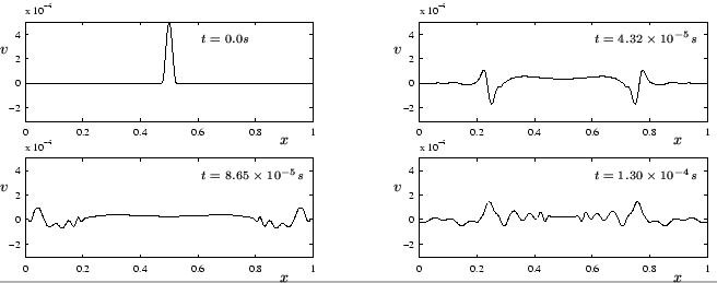 |
Figure 5.14:
Simulation: evolution of the transverse velocity distribution along a Timoshenko beam of linearly-varying thickness, with clamped ends.
|
In both simulations, it is easy to see that due to dispersion, the coherence of the initial velocity distribution is lost; short wavelengths tend to move faster (and hence reflect first from the boundary), as can be seen in the plot at
 s. In the beam with linearly-varying thickness, velocities are amplified in the thin region of the beam, and attenuated in the thick region; the propagation velocities themselves, however, are not significantly altered.
Next: Improved MDKC for Timoshenko's
Up: Timoshenko's Beam Equations
Previous: Boundary Conditions in the
Stefan Bilbao
2002-01-22