Improved MDKC for Timoshenko's System Via Balancing

In the preceding simulation of the steel beam of rectangular cross-section and linearly-varying thickness, we have, from (5.24), $v_{0} = 4.59\times 10^{4}$; the time step is thus restricted to be quite small. We will now show how the balancing or preconditioning approach applied to the (1+1)D transmission line problem in §3.12 can be used to drastically increase the maximum allowable time step for a given grid spacing.

Suppose we scale the dependent variables according to

$$v = r_{1}i_{1}\hspace{0.2in}q = r_{2}i_{2}\hspace{0.2in}\omega = r_{3}i_{3}\hspace{0.2in}m = r_{4}i_{4}$$

and allow the scaling parameters $r_{1},\hdots, r_{4}$ to be arbitrary smooth functions of $x$. Timoshenko's system (5.17)-(5.18) can then be rewritten as

$$\begin{eqnarray}v_{0}\left(\frac{r_{1}}{r_{2}}\right)\rho A \frac... ... &=& \frac{\partial i_{3}}{\partial x}+\frac{r'_{3}}{r_{3}}i_{3} \end{eqnarray}$$ (5.27a)

where primes above the $r_{i}$, $i=1,\hdots, 4$ indicate $x$-differentiation. If we choose:

$$r_{1} = \left(\rho A^{2}G\kappa\right)^{-\frac{1}{4}}\hspace{0.3i... ...ht)^{-\frac{1}{4}}\hspace{0.3in}r_{4} = \left(\rho E I^{2}\right)^{\frac{1}{4}}$$ (5.28)

Then system (5.26) becomes

$$\begin{eqnarray}v_{0}\sqrt{\frac{\rho}{G\kappa}} \frac{\partial i... ... &=& \frac{\partial i_{3}}{\partial x}-\frac{r_{4}'}{r_{4}}i_{3} \end{eqnarray}$$ (5.29a)

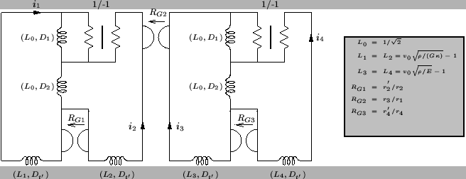
and the constant-proportional terms appear anti-symmetrically (note, from (5.27), that $r_{2}/r_{4} = r_{3}/r_{1}$). In the MDKC shown in Figure 5.15, these terms are all interpreted as gyrator couplings, where the gyrator coefficients are spatially varying. It is easy to check that this system is still symmetric hyperbolic according to definition (3.1).

Figure 5.15: Balanced MDKC for Timoshenko's system.

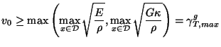
The MDWD network (not shown) implied by the MDKC will be slightly more difficult to program, because of the additional reflection-free ports which will necessarily be introduced, but it has the same memory requirements, and the operation count is slightly larger (due chiefly to the post-scaling of the MDKC currents which must now be performed in order to obtain the physical dependent variables). We now have, however, that

$$v_{0}\geq \max\left(\max_{x\in\mathcal{D}}\sqrt{\frac{E}{\rho}},\max_{x\in\mathcal{D}}\sqrt{\frac{G\kappa}{\rho}}\right) = \gamma_{T, max}^{g}$$

where $\gamma_{T, max}^{g}$ is the maximum group velocity given in (5.20). $v_{0}$ is now optimal (in the CFL sense), for a constant grid spacing. Referring to the simulation of §5.2.5, it is easy to see that that due to the quartic dependence of the moment of inertia $I$ on $x$ (for a beam of linearly varying thickness), the maximum time step allowed by the previous approach (also the maximum time step allowed in [131]) will be severely constrained. Using a balanced formulation and MDKC, we now have $v_{0}=5.10\times 10^{3}$. Thus for a given grid spacing, the maximum time step is now 9 times larger. From a practical standpoint, this is a huge computational advantage.

We repeat that balancing is unnecessary if there is no spatial variation in the problem parameters, and that in a region of the material for which the parameters do not vary, we may simply drop the additional gyrator couplings $R_{G1}$ and $R_{G3}$ from the network entirely. We also note that it is possible to incorporate the scaling of the dependent variables into the MDKC itself by introducing transformers with turn ratios $r_{1},\hdots, r_{4}$ in all the circuit loops; while useful for showing the MD-passivity of the system under scaling, there is no practical reason for doing so.