Plates

The equations of motion of a stiff plate are the (2+1)D generalization of those of a beam. We assume the plate to lie, when at rest, in the $(x,y)$ plane, and to be of thickness $h(x,y)$; the deflection $w(x,y)$ of the plate from its equilibrium state is assumed to be perpendicular to the $(x,y)$ plane. The plate material has density $\rho$, as well as Young's modulus $E$ and Poisson's ratio $\nu$, all of which are assumed, for the sake of generality, to be smooth positive functions of $x$ and $y$. 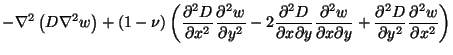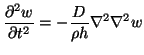In particular, $\nu$ must be less than one-half. The classical development depends on neglecting rotational inertia effects and makes various assumptions analogous to the ``plane sections remain plane and perpendicular to the neutral axis'' hypothesis that was used as the basis for the Euler-Bernoulli beam model [77]. The resulting equation of motion [6,113] can be written as

$$\rho h\frac{\partial^{2}w}{\partial t^{2}} = -\nabla^{2}\left(D\nabla^{2}w\right)+(1-\nu)\left(\frac{\partial^... ...\frac{\partial^{2}D}{\partial y^{2}}\frac{\partial^{2}w}{\partial x^{2}}\right)$$

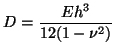
where

$$D = \frac{Eh^{3}}{12(1-\nu^{2})}$$

and used $\nabla^{2} = \frac{\partial^{2}}{\partial x^{2}}+\frac{\partial^{2}}{\partial y^{2}}$. If the material parameters and the thickness are constant, then

$$\frac{\partial^{2}w}{\partial t^{2}} = -\frac{D}{\rho h}\nabla^{2}\nabla^{2}w$$ (5.31)

which is easily seen to be a direct generalization of (5.2). As such, we expect to find the same anomalous behavior of the resulting propagation velocities, which can become infinitely large in the high-frequency limit. Numerical integration of these equations via a waveguide mesh proceeds along exactly the same lines as in the case of the Euler-Bernoulli beam; in particular, we find a restriction on the space step/time step ratio similar to those that resulted in §5.1.2.

Because the development is so similar to the (1+1)D case, we will proceed directly to the more refined model of plate motion, which is a direct generalization of the Timoshenko theory for beams. First proposed by Mindlin, the model [77,120], can be written as system of eight PDEs [173]:

$$\begin{eqnarray}\rho h\frac{\partial v}{\partial t} &=& \frac{\pa... ...l q_{y}}{\partial t} &=& \frac{\partial v}{\partial y}+\omega_{y}\end{eqnarray}$$ (5.32a)

$$\begin{eqnarray}\frac{\rho h^{3}}{12}\frac{\partial \omega_{x}}{\... ...l \omega_{y}}{\partial x}+\frac{\partial \omega_{x}}{\partial y} \end{eqnarray}$$ (5.33a)

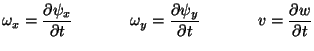
Here, we have written

$$\omega_{x} = \frac{\partial \psi_{x}}{\partial t}\hspace{0.5in}\o... ...c{\partial \psi_{y}}{\partial t}\hspace{0.5in}v = \frac{\partial w}{\partial t}$$

where $w$ is the transverse displacement of the plate, and $(\psi_{x},\psi_{y})$ is the pair of angles giving the orientation of the sides of a deformed differential element of the plate with respect to the perpendicular. (In the classical theory, for which cross-sections of the plate are assumed to remain parallel to the plate normal, we have $(\psi_{x},\psi_{y}) = (-\frac{\partial w}{\partial x}, -\frac{\partial w}{\partial y})$.) In addition, we have the shear forces $(q_{x}, q_{y})$ and moments $(m_{x},m_{y}, m_{xy})$, which are the (2+1)D generalizations of $q$ and $m$. 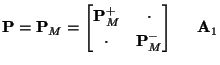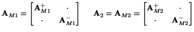The system (5.31)-(5.32) as a whole is known as Mindlin's system, although it is more commonly written s a system of three second-order equations in the variables $w$, $\psi_{x}$ and $\psi_{y}$ [77]. We have written Mindlin's system so that it is easy to see the decomposition into two separate subsystems, one in $(v,q_{x},q_{y})$ and the other in $(\omega_{x}, \omega_{y}, m_{x}, m_{y},m_{xy})$, with the coupling occurring via constant-proportional terms in $\omega_{x}$, $\omega_{y}$, $q_{x}$ and $q_{y}$. In particular, subsystem (5.31) is similar to the lossless parallel-plate system (see §4.4), except for the coupling terms.

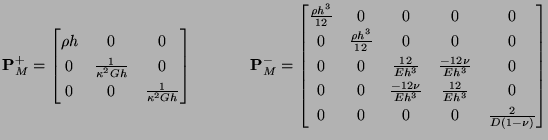
It is easy to see that this system is not, as written, symmetric hyperbolic. It is easy to symmetrize it by taking sums and differences of (5.32c) and (5.32d), in which case we get, in terms of the variable ${\bf w} = [v, q_{x}, q_{y}, \omega_{x}, \omega_{y}, m_{x}, m_{y}, m_{xy}]^{T}$,

$${\bf P} = {\bf P}_{M} = \begin{bmatrix} {\bf P}_{M}^{+}&\cdot\\ \cdot & {\bf P}_{M}^{-}\\ \end{bmatrix}\hspace{0.2in}{\bf A}_{1} = {\bf A}_{M1} = \begin{bmatrix} {\bf A}_{M1}^{+}&\cdot\\ \cdot & ... ...trix} {\bf A}_{M2}^{+}&\cdot\\ \cdot & {\bf A}_{M2}^{-}\\ \end{bmatrix}\notag$$ (5.34)

$$\vspace{0.5in} {\bf B} = {\bf B}_{M} = \begin{bmatrix} \cdot & {\bf B}_{M\times}\\ -{\bf B}_{M\times}^{T} & \cdot\\ \end{bmatrix}$$ (5.35)

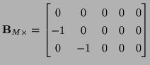
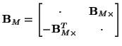
where the $\cdot$ stands for zero entries, and

$${\bf P}_{M}^{+} = \begin{bmatrix}\rho h &0 &0\\ 0 & \frac{1}{\kap... ...12\nu}{Eh^{3}}&\frac{12}{Eh^{3}}&0\\ 0&0&0&0&\frac{2}{D(1-\nu)}\\ \end{bmatrix}$$

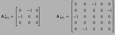$${\bf A}_{M1}^{+} = \begin{bmatrix}0 &-1 &0\\ -1 & 0 & 0\\ 0 & 0 &... ...x}0&0&-1&0&0\\ 0&0&0&0&-1\\ -1&0&0&0&0\\ 0&0&0&0&0\\ 0&-1&0&0&0\\ \end{bmatrix}$$ (5.36)

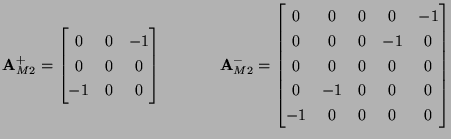$${\bf A}_{M2}^{+} = \begin{bmatrix}0 &0 &-1\\ 0 & 0 & 0\\ -1 & 0 &... ...x}0&0&0&0&-1\\ 0&0&0&-1&0\\ 0&0&0&0&0\\ 0&-1&0&0&0\\ -1&0&0&0&0\\ \end{bmatrix}$$ (5.37)

$${\bf B}_{M\times} = \begin{bmatrix}0 &0 &0&0&0\\ -1 & 0 & 0&0&0\\ 0 & -1 &0&0&0\\ \end{bmatrix}$$

The system defined by (5.33) is lossless, due to the anti-symmetry of ${\bf B}_{M}$. Also, note that ${\bf P}_{M}$ is positive definite (recall that $\nu$ is positive, and less than one-half), but not diagonal; this did not come up in any of the systems we have looked at previously, and will have interesting consequences in the circuit representations in the next section.