


Next: Cylindrical Shells
Up: Plates
Previous: Clamped Edge
Simulation: Mindlin's System, for Plates of Uniform and Varying Thickness
For the sake of illustration, we present two DWN simulations of the vibration of a Mindlin plate. In both cases, the plate is assumed to be square, with side length 1m and to be made of steel; the material parameters are thus
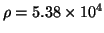 kg/m
kg/m ,
,
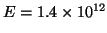 N/m
N/m ,
,
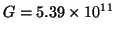 N/m.
N/m.  is taken to be 5/6, and Poisson's ratio
  is set to 0.3. In both cases, the DWN is initialized with a transverse velocity distribution which takes the form of a single lobe of a 2D raised cosine, of radius 0.1m, amplitude
  m/s, and centered at coordinates
  m,
m,  m, where
  m,
m,  m are the coordinates of the bottom left-hand plate corner. The grid spacing is set to be
 cm in the DWN in both cases.
In the first simulation (see Figure 5.21), the plate thickness is 1cm, over the entire plate surface. Boundary conditions are of the free type, given by (5.44a), and implemented as per the DWN termination discussed in the previous section, and shown in Figure 5.20(a). In the second simulation, shown in Figure 5.22, the plate thickness is variable--over most of the plate, it is a constant 1cm, but over the circular region outlined in black (radius 0.2m, and centered at  m,
m,  m), it rises in a raised 2D cosine distribution to a peak of 6cm. In both simulations, snapshots of the transverse velocity distribution are taken every 2.875
 s. The boundary termination is of the clamped type (5.44d) in this case, and has been implemented in the DWN according to Figure 5.20(d).
Light- and dark-colored regions correspond to positive and negative velocities, respectively. The plots have been normalized and interpolated for better visibility. Notice in particular the numerical directional dependence of the propagation velocities at short wavelengths.
Figure 5.21:
DWN simulation of Mindlin's system, for a steel plate of uniform thickness, with free edges.
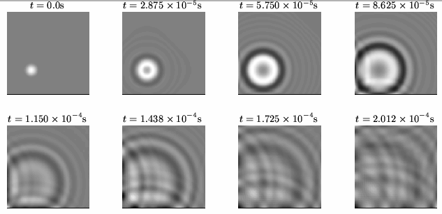 |
Figure 5.22:
DWN simulation of Mindlin's system, for a steel plate of varying thickness. The variation is limited to the interior of the black circles. Boundary conditions are of the clamped type.
|
Next: Cylindrical Shells
Up: Plates
Previous: Clamped Edge
Stefan Bilbao
2002-01-22