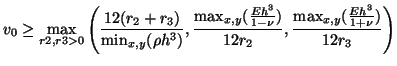
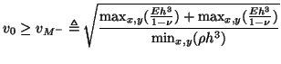
We now introduce scaled dependent variables
Because
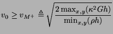
![]() from (5.33) is not diagonal, the coupling between the loops with currents
from (5.33) is not diagonal, the coupling between the loops with currents ![]() and
and ![]() (corresponding to the moments
(corresponding to the moments ![]() and
and ![]() ) is of a type not previously encountered in the systems examined in this thesis. It can be interpreted in terms a coupled inductance between the loops (see §2.3.7); in Figure 5.16, self-inductances are indicated by directed arrows, and mutual inductance by bidirectional arrows. The element values are as indicated in the figure.
) is of a type not previously encountered in the systems examined in this thesis. It can be interpreted in terms a coupled inductance between the loops (see §2.3.7); in Figure 5.16, self-inductances are indicated by directed arrows, and mutual inductance by bidirectional arrows. The element values are as indicated in the figure.
Optimal choices of ![]() ,
, ![]() and
and ![]() , and the optimal stability bound on
, and the optimal stability bound on ![]() are a little more difficult to find in this case. As before, however, they follow from a positivity requirement on the inductance values defined in Figure 5.16. This requirement is simply applied to
are a little more difficult to find in this case. As before, however, they follow from a positivity requirement on the inductance values defined in Figure 5.16. This requirement is simply applied to ![]() ,
, ![]() ,
, ![]() ,
, ![]() ,
, ![]() and
and ![]() , but
, but ![]() and
and ![]() define a coupled inductance between the loops with currents
define a coupled inductance between the loops with currents ![]() and
and ![]() . The coupling matrix will be
. The coupling matrix will be
 |
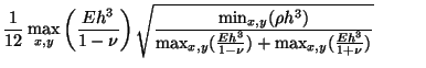
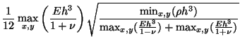
An optimal choice for ![]() is easily shown to be
is easily shown to be
From the positivity requirement on ![]() ,
, ![]() ,
, ![]() , as well as condition (5.36), we have a second bound on
, as well as condition (5.36), we have a second bound on ![]() ,
,
 |
The MDWD network, shown at bottom in Figure 5.16, follows immediately from the MDKC; here, as for the parallel-plate problem discussed in §3.8.1, we have used step sizes
![]() ,
,
![]() . Recall that because coordinate
. Recall that because coordinate
![]() , a step size of
, a step size of
![]() implies a time step of
implies a time step of
![]() , and we have indicated pure time delays of duration
, and we have indicated pure time delays of duration ![]() by
by ![]() . As for the Timoshenko network of Figure 5.6, reflection-free ports will be necessary due to the memoryless gyrator couplings between the loops with currents
. As for the Timoshenko network of Figure 5.6, reflection-free ports will be necessary due to the memoryless gyrator couplings between the loops with currents ![]() and
and ![]() , and
, and ![]() and
and ![]() in the MDKC. The coupled inductance has been treated as a vector scattering junction terminated on a vector inductor, as discussed in §2.3.7. We also note in passing that this network may be balanced in the same way as the Timoshenko system (see §5.2.6) in order to obtain a much better bound on
in the MDKC. The coupled inductance has been treated as a vector scattering junction terminated on a vector inductor, as discussed in §2.3.7. We also note in passing that this network may be balanced in the same way as the Timoshenko system (see §5.2.6) in order to obtain a much better bound on ![]() (at the expense of increased network complexity).
(at the expense of increased network complexity).
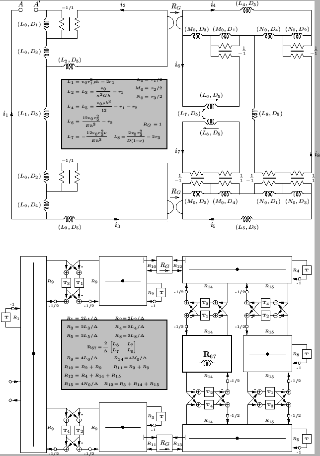
It is also of course possible to put the MDKC into a form which yields, upon discretization, a DWN. This new form is shown in Figure 5.17; now the transverse velocity ![]() and bending moments
and bending moments ![]() ,
, ![]() and
and ![]() are treated as voltages, and inductors in these loops are replaced by gyrators terminated on capacitances. In particular, the coupled inductance in Figure 5.16 is replaced by a coupled capacitance. In order to discretize this MDKC, we apply the trapezoid rule to all the inductances and capacitances with direction
are treated as voltages, and inductors in these loops are replaced by gyrators terminated on capacitances. In particular, the coupled inductance in Figure 5.16 is replaced by a coupled capacitance. In order to discretize this MDKC, we apply the trapezoid rule to all the inductances and capacitances with direction ![]() (using a step size of
(using a step size of
![]() ), and to the Jaumann two-ports, we make use of the alternative spectral mappings defined by (4.109), with step sizes
), and to the Jaumann two-ports, we make use of the alternative spectral mappings defined by (4.109), with step sizes
![]() ,
,
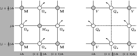
![]() . We have chosen these step sizes such that an interleaved algorithm results; the computational grid is shown in Figure 5.18. Grid quantities (capitalized) are shown next to the points at which they are to be calculated. The grid on the right, which operates on grid functions
. We have chosen these step sizes such that an interleaved algorithm results; the computational grid is shown in Figure 5.18. Grid quantities (capitalized) are shown next to the points at which they are to be calculated. The grid on the right, which operates on grid functions ![]() ,
, ![]() and
and ![]() is identical to the grid for the DWN for the (2+1)D parallel-plate problem (see Figure 4.18), which is to be expected, since the related subnetwork of the MDKC shown in Figure 5.17 is the same as that for the parallel-plate problem (see Figure 4.49). It is coupled via gyrators (these couplings are indicated by curved arrows) to a second grid, over which grid functions
is identical to the grid for the DWN for the (2+1)D parallel-plate problem (see Figure 4.18), which is to be expected, since the related subnetwork of the MDKC shown in Figure 5.17 is the same as that for the parallel-plate problem (see Figure 4.49). It is coupled via gyrators (these couplings are indicated by curved arrows) to a second grid, over which grid functions
![]() ,
,
![]() ,
, ![]() ,
, ![]() and
and ![]() are calculated. In particular,
are calculated. In particular, ![]() and
and ![]() are calculated together as a vector quantity at a vector parallel junction--this vector is written as
are calculated together as a vector quantity at a vector parallel junction--this vector is written as ![]() in Figure 5.18. Waveguide connections (of delay
in Figure 5.18. Waveguide connections (of delay ![]() ) are represented by solid lines, and self-loops and sign-inversions in the signal paths are not shown. Note that at the grey dots, we will have parallel scattering junctions, and at the white dots we will have series junctions; junction quantities are calculated at alternating multiples of
) are represented by solid lines, and self-loops and sign-inversions in the signal paths are not shown. Note that at the grey dots, we will have parallel scattering junctions, and at the white dots we will have series junctions; junction quantities are calculated at alternating multiples of ![]() .
.