The same idea extends simply to the (2+1)D parallel-plate equations (3.67). In this case, we again look at the lossless source-free system, scaled by a factor of ![]() , and can develop an MDKC along the lines of Figure 4.47(b), with
, and can develop an MDKC along the lines of Figure 4.47(b), with ![]() now treated as a voltage instead of a current as in Figure 3.17. We remind the reader that we use the notation
now treated as a voltage instead of a current as in Figure 3.17. We remind the reader that we use the notation ![]() ,
,
![]() in circuit diagrams to indicate directional derivatives in the directions
in circuit diagrams to indicate directional derivatives in the directions ![]() defined by the coordinate transformation (3.22). Also, we have written
defined by the coordinate transformation (3.22). Also, we have written ![]() and
and ![]() for
for ![]() and
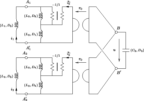
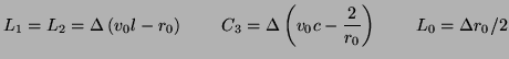
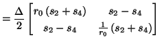
and ![]() , in keeping with the WDF literature [62]. The alternative MDKC is shown in Figure 4.49, and the element values are given by
, in keeping with the WDF literature [62]. The alternative MDKC is shown in Figure 4.49, and the element values are given by
 |
The two two-ports with terminals ![]() ,
, ![]() ,
, ![]() ,
, ![]() and
and ![]() ,
, ![]() ,
, ![]() ,
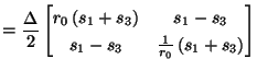
, ![]() are both linear and shift-invariant, and their right-hand pairs of terminals are both connected in parallel with the capacitor. The hybrid matrices for these two-ports are
are both linear and shift-invariant, and their right-hand pairs of terminals are both connected in parallel with the capacitor. The hybrid matrices for these two-ports are
 |
||||
 |
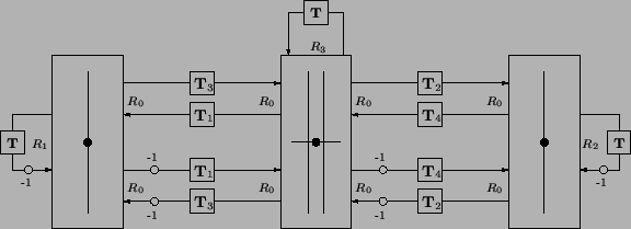 |
When spatial dependence is expanded out, the signal flow graph is identical to the interleaved type III DWN for the parallel-plate equations shown in Figure 4.21, without the loss/source ports. As in (1+1)D, loss and source elements can be reintroduced into the MDKC of Figure 4.49 without difficulty.
It should also be possible to derive DWNs from MDKCs for the same system on alternative grids, such as the hexagonal and triangular grids mentioned in §4.6.1, though we have not investigated this in any detail. In this case, one would presumably begin from the MDKC under the appropriate coordinate transformation. One of these coordinate transformations (which generates a hexagonal grid under uniform sampling in the new coordinates), was discussed briefly in §3.3.3. The full MDKC for the parallel-plate equations in these coordinates is given in [62].