Next: Maxwell's Equations
Up: Incorporating the DWN into
Previous: Alternative MDKC for (2+1)D
Higher-order Accuracy Revisited
Recall that in §3.13, we derived two MDKCs that were suitable for solving the transmission line equations to higher-order spatial accuracy; we were forced, however, to employ a set of alternative spectral mappings very similar to those that have appeared earlier in this section. For this reason, we postponed showing the full scattering network until now. This is a good opportunity to see the flexibility of having a multidimensional representation of a DWN.
The MDKC in Figure 3.25 represents the lossless source-free (1+1)D transmission line equations, in a set of  coordinates defined by (3.21) using the transformation matrix of (3.94). These new coordinates allow us to define directional shifts that refer to points other than nearest neighbors. The general approach to deriving a DWN for this MDKC is the same as in the previous sections; first we perform some network manipulations on the MDKC, and then we apply alternative spectral mappings or integration rules to the connecting LSI two-ports, which then reduce to multidimensional unit elements, which are then interpreted as arrays of digital waveguides. The circuit manipulations in this case are slightly more involved; skipping several steps, we note that we can rewrite the MDKC as shown in Figure 4.51.
Figure 4.51: (a) A modified MDKC for the lossless, source-free(1+1)D transmission line system and (b) a detail of connecting two-ports  ,
, ,
, ,
,  for any
  ,
,
 from (a).
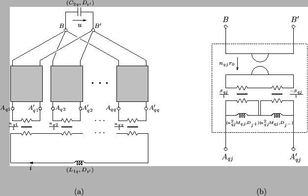 |
As before, we treat  as the voltage across a capacitor, and have introduced a gyrator in each of the connecting two-ports with terminals , , and ,
. In addition, we have extracted a transformer, of turns ratio
as the voltage across a capacitor, and have introduced a gyrator in each of the connecting two-ports with terminals , , and ,
. In addition, we have extracted a transformer, of turns ratio  for each of these two-ports; the gyrator constant is similarly scaled in order to compensate. The effect of this extracted transformer will be to weight the port resistances of the various multidimensional unit elements that result (and hence the waveguide impedances in the resulting DWN). In addition, we will also need to re-scale the inductances from (3.97) by a factor of
  , giving
The two-port shown in Figure 4.51(b) contains two inductors of inductances  defined with respect to the directions
  and
and  . Its continuous hybrid matrix will be, in terms of the two associated complex frequencies
  and
and  ,
,
Under the spectral mappings from and to the frequency domain unit shifts
 and
and
 given by
(which are passive and correspond to the integration rules (3.98), with a shift length of ), the discrete hybrid matrix becomes
It should be clear that in general, this hybrid matrix does not reduce to a pair of series/parallel connected multidimensional unit elements (in which case it should have the form of (4.108), with
and
in place of
 and
and
 ). Under the special choice of
 , however, it does reduce to such a connection, so we have
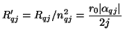
where the port resistances of the unit elements are
The two-port multidimensional unit elements are connected to transformers, of turns ratio , as per Figure 4.51(a). The port resistance at one end of each transformer can be set to that of the unit element to which it is connected, which is  . It is possible to implement these transformers as multiplies by and
  directly in the signal paths, if we make the choice of the other port resistance (which we call
  ) according to the rule discussed in §2.3.4; we thus choose
For the one-port inductor and capacitor (of inductance  and
and  respectively), we use the trapezoid rule with a doubled time step
 , and the wave digital one-ports (of port resistances
 and
and
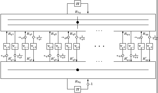
 ) result. The multidimensional network shown in Figure 4.52 can be interpreted as a DWN, and if the parameters
 are chosen according to the method discussed in §3.13, then the DWN will give a
  th-order spatially accurate solution to the (1+1)D lossless source-free transmission line system. In order not to belabor this point any further, we leave the explicit construction of the expanded signal flow graph for this multidimensional DWN from Figure 4.52 (as well as the interleaved DWN which results from the use of coordinates defined by (3.102)) as an exercise to the reader.
Figure:
Multidimensional DWN suitable for a th-order spatially accurate solution to the (1+1)D transmission line equations.
 |
It is interesting that not all DWN topologies permit a higher-order spatially accurate scheme; in §A.2.5, we will look at a stable fourth-order accurate difference scheme for the (2+1)D wave equation which cannot be realized in a straightforward way as a DWN. The topology of the DWN in this section follows directly from a passive MD circuit representation.
Next: Maxwell's Equations
Up: Incorporating the DWN into
Previous: Alternative MDKC for (2+1)D
Stefan Bilbao
2002-01-22