A Fourth-order Scheme

The schemes examined so far have all been spatially accurate to second-order. That is, at any time step, the $L_{2}$ norm of the difference between the numerical solution and the solution to the model problem will be proportional to $\Delta^{2}$. In this section, we examine a family of explicit two-step schemes which are fourth-order spatially accurate. This family is more computationally intensive, due to the fact that updating the grid function requires access to past values which are two grid points away; in addition, we will see that a passive waveguide mesh implementation will not be possible in this case. These disadvantages are mitigated by the fact that the numerical dispersion is greatly reduced, so that the use of a coarse grid may be possible.

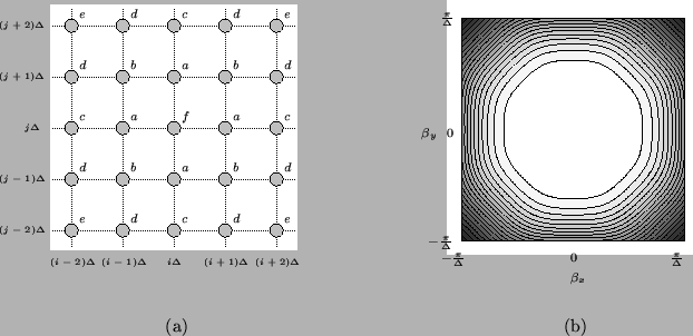
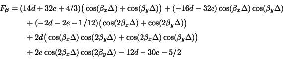
This scheme is, like the standard rectilinear scheme, defined over a grid with indices $i$ and $j$ which refer to a location with coordinates $x=i\Delta$ and $y=j\Delta$. Updating, in this case, at a given point, requires access to values of the grid function at the previous time step at the set of 25 grid points which are located at most $2\Delta$ away in either the $x$ or $y$ directions, as shown in Figure A.7(a). The difference scheme will have the general form

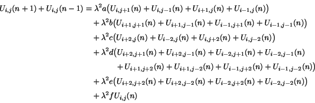$$\begin{split}U_{i,j}(n+1)+U_{i,j}(n-1) &= \lambda^{2}a\big(U_... ...{i-2,j-2}(n)\big)\\ &\quad + \lambda^{2}fU_{i,j}(n) \end{split}$$ (A.25)

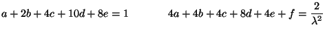
In order for (A.24) to approximate the wave equation, we first require that the constants $a$, $b$, $c$, $d$, $e$ and $f$ satisfy the constraints

$$a+2b+4c+10d+8e = 1\hspace{0.5in}4a+4b+4c+8d+4e+f = \frac{2}{\lambda^{2}}$$ (A.26)

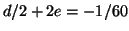
Then, to ensure that the scheme is fourth-order spatially accurate, we additionally require

$$b+8d+16e = 0\hspace{1.0in}a+2b+16c+34d+32e = 0$$ (A.27)

We can then write all the parameters in terms of $d$, $e$ and $\lambda$, as

$$\begin{eqnarray}a &=& 14d+32e+4/3\\ b &=& -8d-16e\\ c &=& -2d-2e-1/12\\ f &=& 2/\lambda^{2}-24d-60e-5 \end{eqnarray}$$ (A.28a)

These constraints are all arrived at through a tedious but straightforward Taylor series expansion of the scheme. As for the interpolated scheme discussed in §A.2.2, passivity is guaranteed by a simple positivity condition on the scheme parameters, in this case $a,\hdots,f$. From (A.27c), it should be clear that if $d\geq 0$ and $e\geq 0$, then we must necessarily have $c\leq -1/12$, and a passive waveguide mesh implementation for this scheme is ruled out. This is not to say that fourth-order spatially accurate DWNs do not exist; we showed, in §4.10.5 that such a network does exist, at least in the case of the (1+1)D transmission line system (the wave equation is a special case of this system). The conclusion is that the topology of the form discussed in this section does not permit a mesh realization, but there are other forms that do.

The amplification polynomial for this scheme is of the form of (A.5), with 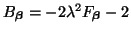$B_{\mbox{{\scriptsize\boldmath $\beta$}}} = -2\lambda^{2}F_{\mbox{{\scriptsize\boldmath $\beta$}}}-2$ and

$$\begin{split}F_{\mbox{{\scriptsize\boldmath$\beta$}}} &= (14d... ...2\beta_{x}\Delta)\cos(2\beta_{y}\Delta)-12d-30e-5/2 \end{split}$$

In order to determine stability bounds, we are faced with finding the extrema of $F_{\mbox{{\scriptsize\boldmath $\beta$}}}$ in terms of the parameters $d$ and $e$. Because $F_{\mbox{{\scriptsize\boldmath $\beta$}}}$ is not multilinear in the cosines, finding these extrema explicitly is a challenging problem.

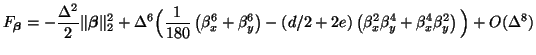
Let us first simplify the class of difference schemes by looking for those which exhibit maximally direction-independent numerical dispersion. As in §A.2.2, we expand $F_{\mbox{{\scriptsize\boldmath $\beta$}}}$ in a Taylor series about $\beta$$={\bf0}$, to get

$$F_{\mbox{{\scriptsize\boldmath$\beta$}}} = -\frac{\Delta^{2}}{2}\... ...\beta_{x}^{2}\beta_{y}^{4}+\beta_{x}^{4}\beta_{y}^{2}\right)\Big)+O(\Delta^{8})$$

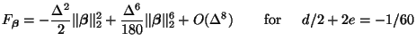
The absence of a term in $\Delta^{4}$ reflects the fourth-order accuracy of the scheme. If we choose $d/2+2e = -1/60$, however, we get

$$F_{\mbox{{\scriptsize\boldmath$\beta$}}} = -\frac{\Delta^{2}}{2}\... ...{2}^{6}+O(\Delta^{8})\hspace{0.3in}\mbox{{\rm for}}\hspace{0.2in}d/2+2e = -1/60$$

and the scheme is direction-independent to sixth order in $\Delta$.

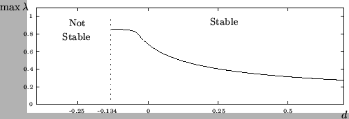
Making use of this setting for $e$ in terms of $d$, $F_{\mbox{{\scriptsize\boldmath $\beta$}}}$ now depends only on the free parameter $d$; through a computer analysis, it is possible to show that condition (A.8) is satisfied for $d>-0.134$. The upper bound on $\lambda$, from condition (A.9) is plotted as a function of $d$ in Figure A.6.

Figure A.6: Stability bound for the fourth-order scheme (A.24), as a function of the free parameter $d$, in the optimally direction-independent case. The solid line indicates the maximum value of $\lambda$ for a given value of $d$. The scheme is stable only for $d>-0.134$.

We have plotted a numerical dispersion profile in Figure A.7(b). It is interesting to note that the maximum value of $v_{\mbox{{\scriptsize\boldmath$\beta$}}, phase}/\gamma$ for this family of schemes would always appear to be slightly greater than 1, although the numerical phase velocity does indeed approach the physical velocity at spatial DC (as it will for any consistent scheme).

Figure A.7: The fourth-order spatially accurate scheme (A.24)-- (a) numerical grid, where the letters $a$ through $f$ refer to the related coefficients from (A.24); (b) $v_{\mbox{{\scriptsize\boldmath$\beta$}}, phase}/\gamma$ for the scheme at for $d=-0.044$ and $\lambda = 0.6174$, which is away from the bound shown in Figure A.6. $v_{\mbox{{\scriptsize\boldmath$\beta$}}, phase}/\gamma$ takes on a maximum of 1.0144 (not shown).

The computational and add densities for this scheme are, in general,

$$\rho_{fourth} = \frac{v_{0}}{\Delta^{3}}\hspace{1.0in}\sigma_{fourth} = \frac{25v_{0}}{\Delta^{3}}\hspace{0.3in}$$

There are several ways of cutting down on computational costs; for example, because $d$ and $e$ are free parameters, we may simply set them to zero, and the add density is significantly reduced. There is, however, no decomposition of this scheme into mutually exclusive subschemes.