The Hexagonal Scheme

The hexagonal scheme is different from those previously discussed in that updating is not the same at every point on the grid. Indeed, one-half the grid points have a ``mirror-image'' orientation with respect to the other half, as shown in Figure A.5(a). For this reason, we will take special care in the analysis of this system; first suppose that we have two grid functions $U_{1}(n)$ and $U_{2}(n)$ defined over the two subgrids (labeled 1 and 2, in Figure A.5). We index these two grid functions as $U_{1,i,j}(n)$ and $U_{2,i+2,j}(n)$, for $i$ and $j$ integer such that $i=3m$, for integer $m$, and $j+i/3$ is even. $U_{1,i,j}(n)$ will serve as an approximation to some continuous function $u_{1}$ at the point $(x=\Delta i/2, y=\sqrt{3}j\Delta/2, t=nT)$, and $U_{2,i+2,j}(n)$ will approximate a function $u_{2}$ at a point with coordinates $(x=\Delta i/2+\Delta, y = \sqrt{3}j\Delta/2, t=nT)$. As before the distance between any grid point and its nearest neighbors (three in this case) is $\Delta$. The difference scheme for the hexagonal waveguide mesh can then be written as the system

$$\begin{eqnarray}U_{1,i,j}(n+1)+U_{1,i,j}(n-1) &=& \frac{4}{3}\lam... ...(n)\Big)\notag\\ && + 2\left(1-2\lambda^{2}\right)U_{2,i+2,j}(n) \end{eqnarray}$$

Consistency of (A.20) with the wave equation is not immediately apparent. We can check it as follows. First expand (A.20) in a Taylor series in terms of the continuous functions $u_{1}$ and $u_{2}$ to get

$$\left(T^{2}\frac{\partial^{2}}{\partial t^{2}} +4\lambda^{2}\right)u_{1} = \lambda^{2}\left(4+\Delta^{2}\nabla^{2}\right)u_{2}$$

$$\left(T^{2}\frac{\partial^{2}}{\partial t^{2}} +4\lambda^{2}\right)u_{2} = \lambda^{2}\left(4+\Delta^{2}\nabla^{2}\right)u_{1}$$

to $O(\Delta^{4}, T^{4})$. This system can then be reduced to

$$\left(T^{2}\frac{\partial^{2}}{\partial t^{2}} +4\lambda^{2}\right)^{2}u = \lambda^{4}\left(4+\Delta^{2}\nabla^{2}\right)^{2}u$$

where $u$ is either of $u_{1}$ or $u_{2}$. Discarding higher order terms in $T$ and $\Delta$ gives the wave equation.

In terms of the spatial Fourier spectra of the grid functions $U_{1}$ and $U_{2}$, we may write the differencing system (A.20) in the vector form of (A.10) with

$$\hat{\bf U}_{\mbox{{\scriptsize\boldmath$\beta$}}} = \begin{bmatr... ...i_{\mbox{{\scriptsize\boldmath$\beta$}}}^{*}&-2(1-2\lambda^{2})\\ \end{bmatrix}$$

where

$$\psi_{\mbox{{\scriptsize\boldmath$\beta$}}} = e^{i\beta_{x}\Delta}+2e^{-i\beta_{x}\Delta/2}\cos(\sqrt{3}\beta_{y}\Delta/2)$$

Because ${\bf B}_{\mbox{{\scriptsize\boldmath $\beta$}}}$ is Hermitian, we can then change variables so that the system is the form of (A.11), with

$$\mbox{\boldmath$\Lambda$} _{\mbox{{\scriptsize\boldmath$\beta$}}} = \begin{bmatrix}-2(1-2\l... ...lambda^{2}\vert\psi_{\mbox{{\scriptsize\boldmath$\beta$}}}\vert\\ \end{bmatrix}$$

The necessary stability condition, from (A.12) will then be

$$\max_{\mbox{{\scriptsize\boldmath$\beta$}}}\vert-2(1-2\lambda^{2}... ...}{3}\lambda^{2}\vert\psi_{\mbox{{\scriptsize\boldmath$\beta$}}}\vert\vert\leq 2$$ (A.22)

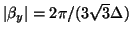It is easy to check that $\vert\psi_{\mbox{{\scriptsize\boldmath $\beta$}}}\vert$ takes on a maximum of 3 when $\beta_{x}=\beta_{y}=0$, and is minimized for $\beta_{x} = 0$, $\vert\beta_{y}\vert = 4\pi/(3\sqrt{3}\Delta)$ and for $\vert\beta_{x}\vert = 2\pi/3$, $\vert\beta_{y}\vert = 2\pi/(3\sqrt{3}\Delta)$, where it takes on the value 0. It is then easy to show that we require $\lambda\leq 1/\sqrt{2}$ in order to satisfy (A.21). This coincides with the passivity bound, from (4.79).

An analysis of numerical dispersion is more complex in the vector case. Beginning from the uncoupled system defined by $\Lambda$$_{\mbox{{\scriptsize\boldmath $\beta$}}}$, whose upper and lower diagonal entries we will call $\Lambda_{\mbox{{\scriptsize\boldmath $\beta$}},1}$ and $\Lambda_{\mbox{{\scriptsize\boldmath $\beta$}},2}$ respectively, we can see that we will thus have two pairs of spectral amplification factors, one for each uncoupled scalar equation. These will be given by

$$G_{\mbox{{\scriptsize\boldmath$\beta$}},1,\pm} = \frac{1}{2}\left... ...ta$}},2}\pm\sqrt{\Lambda_{\mbox{{\scriptsize\boldmath$\beta$}},2}^{2}-4}\right)$$

It is useful to check the values of the amplification factors at the spatial DC frequency, and at the stability bound, where we have $\Lambda_{\mbox{{\scriptsize\boldmath $\beta$}},1} = 2$, $\Lambda_{\mbox{{\scriptsize\boldmath $\beta$}},2} = -2$. At this frequency, the spectral amplification factors take on the values

$$G_{\mbox{{\scriptsize\boldmath$\beta$}}=0,1,\pm} = -1\hspace{0.5in}G_{\mbox{{\scriptsize\boldmath$\beta$}}=0,2,\pm} = 1$$ (A.23)

Clearly, the pair of spectral amplification factors $G_{\mbox{{\scriptsize\boldmath $\beta$}}=0,2,\pm}$ correctly represents wave propagation at spatial DC, but the factors $G_{\mbox{{\scriptsize\boldmath $\beta$}}=0,1,\pm}$ will be responsible for parasitic oscillations [176] in the hexagonal scheme; they will not, in general, be overly problematic, since the energy allowed into such modes must vanish as the grid spacing $\Delta$ is decreased; this is a result of the consistency of the numerical scheme (A.20) with the wave equation, as was shown earlier in this subsection. In order to clarify this point, it is useful to examine the diagonalizing transformation defined by ${\bf J}_{\mbox{{\scriptsize\boldmath $\beta$}}}$, which takes the Fourier-transformed hexagonal scheme in the form of (A.10), in the variable $\hat{{\bf U}}_{\mbox{{\scriptsize\boldmath $\beta$}}}$, to that of (A.11), in $\hat{{\bf V}}_{\mbox{{\scriptsize\boldmath $\beta$}}}$. At $\beta$$=0$, and for $\lambda =1/\sqrt{2}$, we have

$${\bf B}_{\mbox{{\scriptsize\boldmath$\beta$}}=0} = \begin{bmatrix... ...egin{bmatrix}\hspace{0.05in}\!\!-1&1\\ \hspace{0.05in}\,\,\,1&1\\ \end{bmatrix}$$

and thus $\hat{V}_{1,\mbox{{\scriptsize\boldmath $\beta$}}=0} = (-\hat{U}_{1,\mbox{{\scr... ...math $\beta$}}=0}+\hat{U}_{2,\mbox{{\scriptsize\boldmath $\beta$}}=0})/\sqrt{2}$ and $\hat{V}_{2,\mbox{{\scriptsize\boldmath $\beta$}}=0} = (\hat{U}_{1,\mbox{{\scri... ...math $\beta$}}=0}+\hat{U}_{2,\mbox{{\scriptsize\boldmath $\beta$}}=0})/\sqrt{2}$. Because scheme (A.20) is consistent with the wave equation, then for any reasonable choice of initial conditions, we must have that $\hat{U}_{1,\mbox{{\scriptsize\boldmath $\beta$}}=0}\approx\hat{U}_{2,\mbox{{\scriptsize\boldmath $\beta$}}=0}$, as $\Delta$ becomes small. Thus $\hat{V}_{1,\mbox{{\scriptsize\boldmath $\beta$}}=0}$, the component of the numerical solution whose spectral amplification is governed by the parasitic factor $G_{\mbox{{\scriptsize\boldmath $\beta$}}=0,1,\pm}$ must vanish in this limit as well.

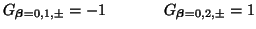
Figure A.5: The hexagonal scheme (A.20)-- (a) numerical grid and connections, where grey/white coloration of points indicates a division into mutually exclusive sub schemes at the stability bound; (b) $v_{\mbox{{\scriptsize\boldmath$\beta$}}, phase}/\gamma$ for the scheme at the passivity bound, $\lambda =1/\sqrt{2}$, for the dominant mode.

The computational and add densities, for the general scheme (A.20), and at the stability limit for $\lambda =1/\sqrt{2}$ will be given by

$$\rho_{hex} = \frac{4v_{0}}{3\sqrt{3}\Delta^{3}} \sigma_{hex} = \frac{16v_{0}}{3\sqrt{3}\Delta^{3}}$$

$$\rho^{s}_{hex} = \frac{2\sqrt{2}\gamma}{3\sqrt{3}\Delta^{3}} \sigma^{s}_{hex} = \frac{2\sqrt{2}\gamma}{\sqrt{3}\Delta^{3}}$$

As in the rectilinear scheme, we have used the fact that the hexagonal scheme decouples into two independent subschemes at the stability limit.

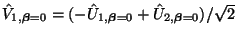
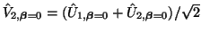
One other point is worthy of comment. Consider again the vector equation which describes the time evolution of the spatial spectra for the hexagonal scheme, which, in diagonalized form, is exactly (A.11). At the stability limit, then, for $\lambda =1/\sqrt{2}$, we will have

$$\mbox{\boldmath$\Lambda$} _{\mbox{{\scriptsize\boldmath$\beta$}}} = \begin{bmatrix}\frac{2}... ...frac{2}{3}\vert\psi_{\mbox{{\scriptsize\boldmath$\beta$}}}\vert\\ \end{bmatrix}$$

Let us examine the second uncoupled subsystem. From (A.22), the spectral amplification factors will then be

$$G_{\mbox{{\scriptsize\boldmath$\beta$}},2,\pm} = \frac{1}{3}\vert... ...vert\psi_{\mbox{{\scriptsize\boldmath$\beta$}}}\vert^{2}-1\right)^{\frac{1}{2}}$$

It is of interest to see the effect of the amplification factors after two time steps; these will simply be the squares of $G_{\mbox{{\scriptsize\boldmath $\beta$}},2,\pm}$, which are

$$G_{\mbox{{\scriptsize\boldmath$\beta$}},2,\pm}^{2} = -1+\frac{2}{... ...vert\psi_{\mbox{{\scriptsize\boldmath$\beta$}}}\vert^{2}-1\right)^{\frac{1}{2}}$$ (A.24)

The important point here is that the two-step spectral amplification factors for scheme (A.20) are identical to the one-step factor for the triangular scheme with grid spacing $\sqrt{3}\Delta$ at its own stability limit; these factors were given in (A.19). This is perhaps not surprising, given that, from Figure A.5(a), it is clear that that either of the two sub grids for the hexagonal scheme forms a triangular grid of spacing $\sqrt{3}\Delta$. What is surprising is that a triangular waveguide mesh at the stability limit is not a concretely passive structure (see previous section). That is to say, it will still operate stably (in the Von Neumann sense), but will require negative self-loop immittances. Thus a hexagonal waveguide mesh, at its passivity/stability bound can be seen as a passive realization of the stable difference scheme on a triangular grid. The question as to whether there is always a passive realization for any stable difference scheme remains open.