Multi-step Schemes

Multi-step methods can be treated in a very similar way. An explicit $M$-step method is defined by

$$U_{{\bf m}}(n+1) = \sum_{r=1}^{M}\sum_{{\bf k}\in \mathbb{K}_{r}}\alpha_{{\bf k}}U_{{\bf m - k}}(n+1-r)$$

for constant coefficients $\alpha_{{\bf k}}$ contained in subsets $\mathbb{K}_{r}$ of $\mathbb{Z}^{N}$. Taking the Fourier transform of this recursion gives

$$\hat{U}_{\mbox{{\scriptsize\boldmath$\beta$}}}(n+1) = \sum_{r=1}^... ...iptsize\boldmath$\beta$}}}\hat{U}_{\mbox{{\scriptsize\boldmath$\beta$}}}(n+1-r)$$ (A.5)

A simple way of examining (A.4) is to look for solutions of the form $\hat{U}_{\mbox{{\scriptsize\boldmath $\beta$}}}(q) = G_{\mbox{{\scriptsize\boldmath $\beta$}}}^{q}\hat{U}_{\mbox{{\scriptsize\boldmath $\beta$}}}(0)$. This gives the amplification polynomial equation

$$G_{\mbox{{\scriptsize\boldmath$\beta$}}}^{M} = \sum_{r=1}^{M}\sum... ...x{{\scriptsize\boldmath$\beta$}}}G_{\mbox{{\scriptsize\boldmath$\beta$}}}^{M-r}$$

the solutions of which, $G_{\mbox{{\scriptsize\boldmath $\beta$}}, \nu}$, $\nu = 1,\hdots,M$ must be bounded by unity for stability (though in general, this is not sufficient, as we will show presently for a special case).

A particular form of the amplification polynomial equation which will appear frequently in our subsequent treatment of finite difference schemes for the wave equation is that of a simple two-step centered difference approximation, namely

$$G_{\mbox{{\scriptsize\boldmath$\beta$}}}^{2}+B_{\mbox{{\scriptsize\boldmath$\beta$}}}G_{\mbox{{\scriptsize\boldmath$\beta$}}}+1 = 0$$ (A.6)

for some real function $B_{\mbox{{\scriptsize\boldmath $\beta$}}}$. This expression has solutions

$$G_{\mbox{{\scriptsize\boldmath$\beta$}}, \pm} = \frac{1}{2}\left(... ...ldmath$\beta$}}}\pm\sqrt{B_{\mbox{{\scriptsize\boldmath$\beta$}}}^{2}-4}\right)$$ (A.7)

which will be bounded by (and in fact equal to) unity in magnitude if we have $\vert B_{\mbox{{\scriptsize\boldmath $\beta$}}}\vert\leq 2$ for all $\beta$. Furthermore, if $\vert B_{\mbox{{\scriptsize\boldmath $\beta$}}}\vert>2$ for some $\beta$, then we will necessarily have an amplification factor with magnitude greater than one at that frequency. For any $\beta$ for which $G_{\mbox{{\scriptsize\boldmath $\beta$}}, \pm}$ are not equal, we can write

$$\hat{U}_{\mbox{{\scriptsize\boldmath$\beta$}}}(n+1) = \frac{G_{\m... ...iptsize\boldmath$\beta$}}, -}}G_{\mbox{{\scriptsize\boldmath$\beta$}}, -}^{n+1}$$

where $\hat{U}_{\mbox{{\scriptsize\boldmath $\beta$}},0}$ and $\hat{U}_{\mbox{{\scriptsize\boldmath $\beta$}},1}$ are the spatial frequency spectra of the two grid functions (at time steps $n=0$ and $n=1$) used to initialize the two-step method. It is easy to show that the $L_{2}$ norm of $U_{{\bf m}}(n)$ can be bounded in terms of the norms of the initial conditions if the spectral amplification factors are distinct and bounded by 1 in magnitude at all wavenumbers.

It is important to realize, however, that the condition that these roots $G_{\mbox{{\scriptsize\boldmath $\beta$}}, \pm}$ be bounded by unity is necessary, but not sufficient to ensure no growth in the $L_{2}$ norm of the solution; this point has not been addressed in the finite difference treatment of waveguide meshes. In fact, as shown in §4.3.4, the simple centered difference approximation to the wave equation admits linearly growing solutions.

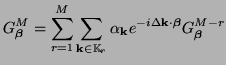
This behavior can be examined in the spectral domain as we will now show, as per [176]. Notice that the solutions (A.6) of the amplification polynomial equation for the two-step scheme can coincide if, and only if at some frequency $\beta$$=$   $\beta$$_{0}$, $B_{\mbox{{\scriptsize\boldmath $\beta_{0}$}}} = \pm 2$, in which case we have $G_{\mbox{{\scriptsize\boldmath $\beta_{0}$}}, +} =G_{\mbox{{\scriptsize\boldmath $\beta_{0}$}}, -} = \mp 1$. The evolution of the particular spatial frequency component at frequency $\beta$$_{0}$ can be written as

$$\hat{U}_{\mbox{{\scriptsize\boldmath$\beta_{0}$}}}(n) = (\mp 1)^{... ...h$\beta_{0}$}},1}\pm\hat{U}_{\mbox{{\scriptsize\boldmath$\beta_{0}$}},0}\right)$$

We can thus expect some linear growth at any such frequency $\beta$$_{0}$ if we do not properly initialize the algorithm, so as to cancel the linearly growing part of the solution. It also follows that in employing such a method, one may need to be particularly careful when applying an excitation which contains such frequency components, and that nonlinear signal quantization may pump energy into such modes, even if none is originally present there.

Strikwerda does not classify such linear growth as unstable, because the wave equation itself admits, in addition to traveling wave solutions, a solution which grows linearly with time. For the physical modeling of musical instruments and acoustic spaces, however (the problems to which finite difference schemes of the form to be discussed shortly are often applied), such solutions are nonphysical and definitely not acceptable. These comments concerning this mild linear instability apply to schemes in unbounded domains; when boundary conditions are present, further analysis will be required.

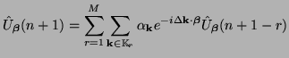
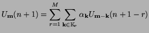
In order to simplify the analysis of these schemes, we mention that for difference schemes for the wave equation, it is often possible to write

$$B_{\mbox{{\scriptsize\boldmath$\beta$}}} = -2\lambda^{2}F_{\mbox{{\scriptsize\boldmath$\beta$}}}-2$$ (A.8)

where $\lambda^{2}\triangleq \gamma^{2}/v_{0}^{2}$ and $F_{\mbox{{\scriptsize\boldmath $\beta$}}}$ is independent of $\lambda$. In this case, the stability condition can be rewritten as

$$\max_{\mbox{{\scriptsize\boldmath$\beta$}}}\vert B_{\mbox{{\scrip... ...$\beta$}}}\vert\lambda^{2}F_{\mbox{{\scriptsize\boldmath$\beta$}}}+1\vert\leq 1$$

This new condition on $F_{\mbox{{\scriptsize\boldmath $\beta$}}}$ is easier to analyze: we first require

$$\max_{\mbox{{\scriptsize\boldmath$\beta$}}}F_{\mbox{{\scriptsize\boldmath$\beta$}}}\leq 0\hspace{0.5in}$$ (A.9)

and if (A.8) holds, we get a further bound on $\lambda$, namely

$$\lambda\leq \sqrt{\frac{-2}{\min_{\mbox{{\scriptsize\boldmath$\be... ...\mbox{{\scriptsize\boldmath$\beta$}}}F_{\mbox{{\scriptsize\boldmath$\beta$}}}}}$$ (A.10)

Thus the stability of these schemes can be simply analyzed in terms of the global maximum and minimum of $F_{\mbox{{\scriptsize\boldmath $\beta$}}}$.

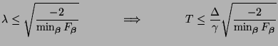
For certain schemes (in particular, the interpolated schemes to be discussed in §A.2.2 and §A.3.3), the function $F_{\mbox{{\scriptsize\boldmath $\beta$}}}$ depends on several parameters. Condition (A.8) tells us the the range of parameters over which our scheme is stable, and over the stability region, condition (A.9) gives us a maximum time step $T$, in terms of the grid spacing $\Delta$.