The (3+1)D Interpolated Rectilinear Scheme

In the interest of achieving a more uniform numerical dispersion profile in (3+1)D, it is of course possible to define an interpolated scheme [155,158], in the same way as was done in (2+1)D in §A.2.2. We will again have a two-step scheme, and updating at a given grid point is performed with reference to, at the previous time step, the grid point at the same location, as well as the 26 nearest neighbors: the six points a distance $\Delta$ away, twelve points at a distance of $\sqrt{2}\Delta$, and eight points that are $\sqrt{3}\Delta$ away--see Figure A.11(a). We present here a complete analysis of the relevant stability conditions, as well as the conditions under which a waveguide mesh implementation exists. We also look at a means of minimizing directional dependence of the numerical dispersion.

Like the cubic rectilinear and octahedral schemes, this scheme will be defined over a rectilinear grid indexed by $i$, $j$ and $k$ and will have the general form

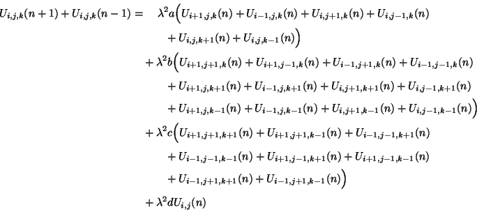$$\begin{split}U_{i,j,k}(n+1)+U_{i,j,k}(n-1) &= \quad \lambda^{... ...+1,k-1}(n)\Big)\\ &\quad + \lambda^{2}dU_{i,j}(n)\\ \end{split}$$ (A.31)

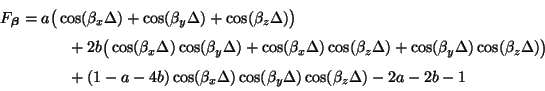
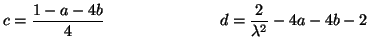
In order for scheme (A.30) to satisfy the wave equation, we require the constants $a$, $b$, $c$ and $d$ to satisfy the constraints

$$c = \frac{1-a-4b}{4}\hspace{1.0in}d = \frac{2}{\lambda^{2}}-4a-4b-2$$ (A.32)

and a family of difference schemes parametrized by $a$, $b$ and $\lambda$ results.

The stability analysis of this scheme proceeds along the same lines as that of the (2+1)D scheme, though as we shall see, the stability condition on the parameters $a$ and $b$ is considerably more complex. As before, we have an amplification polynomial of the form of (A.5), now with

$$\begin{split}F_{\mbox{{\scriptsize\boldmath$\beta$}}} &= a\bi... ...)\cos(\beta_{y}\Delta)\cos(\beta_{z}\Delta)-2a-2b-1 \end{split}$$

where as before, 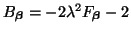$B_{\mbox{{\scriptsize\boldmath $\beta$}}} = -2\lambda^{2}F_{\mbox{{\scriptsize\boldmath $\beta$}}}-2$. Because $F_{\mbox{{\scriptsize\boldmath $\beta$}}}$ is again multilinear in the three cosines, its extrema can only occur at the eight corners of the cubic region defined by $\vert\cos(\beta_{x}\Delta)\vert\leq 1$, $\vert\cos(\beta_{y}\Delta)\vert\leq 1$ and $\vert\cos(\beta_{z}\Delta)\vert\leq 1$. These extrema are

$$F_{\mbox{{\scriptsize\boldmath$\beta$}}^{T} = [0,0,0]} = 0\notag$$

$$F_{\mbox{{\scriptsize\boldmath$\beta$}}^{T} = [\pi/\Delta,0,0]} =... ...pi/\Delta,0]} = F_{\mbox{{\scriptsize\boldmath$\beta$}}^{T} = [0,0,\pi/\Delta]} = -2\notag$$

$$F_{\mbox{{\scriptsize\boldmath$\beta$}}^{T} = [\pi/\Delta,\pi/\De... ...ta]} = F_{\mbox{{\scriptsize\boldmath$\beta$}}^{T} = [\pi/\Delta,\pi/\Delta,0]} = -4a-8b\notag$$

$$F_{\mbox{{\scriptsize\boldmath$\beta$}}^{T} = [\pi/\Delta,\pi/\Delta,\pi/\Delta]} = -4a+8b-2$$

The non-positivity requirement on $F_{\mbox{{\scriptsize\boldmath $\beta$}}}$ then amounts to requiring that these extreme values be non-positive. The resulting stability region in the $(a,b)$ plane is shown in grey in Figure A.10(a).

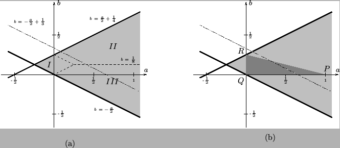
Figure A.10: (a) Stability region, in grey, for the interpolated rectilinear scheme, plotted in the $(a,b)$ plane. This region can be divided into three sub-regions, labeled $I$, $II$, and $III$ separated by dashed lines, over which different stability conditions on $\lambda$ apply. In region $I$, we must have $\lambda\leq 1$, in region $II$ $\lambda \leq 1/\sqrt{2a+4b}$, and in region $III$ $\lambda\leq 1/\sqrt{2a-4b+1}$. The dotted line indicates choices of $a$ and $b$ for which numerical dispersion is optimally direction-independent. (b) The subset of stable schemes for which a passive waveguide mesh implementation exists is shown in dark grey. Over this region, we require $\lambda\leq 1/\sqrt{2a+2b+1}$. This bound is more strict than the stability conditions mentioned above in the same region. We also remark that this interpolated scheme reduces to other simpler schemes under particular choices of $a$ and $b$. At point $P$, we have the cubic rectilinear scheme (see §A.3.1), at point $Q$ we have the octahedral scheme (see §A.3.2), and at point $R$ we have what might be called a ``dodecahedral'' scheme. Notice in particular that none of these schemes is optimally direction-independent (i.e., $P$, $Q$ and $R$ do not lie on the dotted line).

Assuming that $a$ and $b$ fall in this region, we must now find the values of $\lambda$ which satisfy (A.9). The minimum value of $F_{\mbox{{\scriptsize\boldmath $\beta$}}}$ depends on $a$ and $b$ in a non-trivial way; referring to Figure A.10(a), the stability domain can be divided into three regions, and in each there is a different closed form expression for the upper bound on $\lambda$. These bounds are given explicitly in the caption to Figure A.10(a).

In order to examine the directional dependence of the dispersion error, we may expand $F_{\mbox{{\scriptsize\boldmath $\beta$}}}$ in a Taylor series about $\beta$$={\bf0}$, as was done in the (2+1)D case. We have

$$F_{\mbox{{\scriptsize\boldmath$\beta$}}} = -\Delta^{2}\Vert\mbox{... ...beta_{x}^{2}\beta_{z}^{2}+\beta_{y}^{2}\beta_{z}^{2}\right)\Big) +O(\Delta^{6})$$

which implies that

$$F_{\mbox{{\scriptsize\boldmath$\beta$}}} = -\Delta^{2}\Vert\mbox{... ...t _{2}^{4} +O(\Delta^{6})\hspace{1.0in}\mbox{{\rm for}}\hspace{0.1in}b=-a/2+1/3$$

and the dispersion error is directionally-independent to fourth order. This special choice of the parameters $a$ and $b$ is plotted as a dotted line in Figure A.10(a). It is well worth comparing this optimization method with the computer-based techniques applied to the same problem in [158].

The computational and add densities for the scheme will be

$$\rho_{3Dinterp} = \frac{v_{0}}{\Delta^{4}}\hspace{1.0in}\sigma_{3Dinterp} = \frac{27v_{0}}{\Delta^{4}}$$

Considerable computational savings are possible if any of $a$, $b$, $c$ or $d$ is zero.

Finally, we remark that the (3+1)D interpolated scheme can be realized as a waveguide mesh, where, at any given junction, we will have four types of waveguide connections: those of admittances $Y_{a}$, $Y_{b}$ and $Y_{c}$ are connected to the neighboring junctions located at gridpoints at distances $\Delta$, $\sqrt{2}\Delta$ and $\sqrt{3}\Delta$ away respectively, and a self-loop of admittance $Y_{d}$ is also connected to every junction. We end up with exactly difference scheme (A.30), with

$$\lambda^{2}a = \frac{2Y_{a}}{Y_{J}}\hspace{0.3in}\lambda^{2}b = \... ...da^{2}d = \frac{2Y_{d}}{Y_{J}}\hspace{0.5in}Y_{J} = 6Y_{a}+12Y_{b}+8Y_{c}+Y_{d}$$

The passivity condition is then a positivity condition on these admittances, and thus on the parameters $a$, $b$, $c$ and $d$. Recalling the expression for $c$ in terms of $a$ and $b$ from (A.31), we must have

$$a\geq 0\hspace{0.2in}b\geq 0\hspace{0.2in}b\leq\frac{1-a}{4}$$

This region is shown, in dark grey, in Figure A.10(b). The positivity condition on $d$ (expressed in terms of $a$, $b$ and $\lambda$ as per (A.31)) gives the bound on $\lambda$, which is

$$\lambda \leq \sqrt{\frac{1}{2a+2b+1}}$$

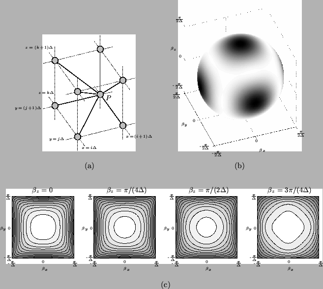
Figure A.11: The (3+1)D interpolated rectilinear scheme (A.30)-- (a) numerical grid and connections, from a central grid point (labeled P) to its neighbors in one octant. (b) $v_{\mbox{{\scriptsize\boldmath$\beta$}}, phase}/\gamma$ for the scheme with $a=0.42$ and $b=0.1233$ at the stability bound $\lambda = 0.8617$, for a spherical surface with $\Vert$$\beta$$\Vert _{2} = \pi/(2\Delta)$--the shading is normalized over the surface so that white and black refer to minimal and maximal dispersion error, respectively. Here, unlike for the cubic rectilinear and octahedral schemes, there are no dispersionless directions. The variation in the numerical phase velocity is, however, quite small, ranging from 96.81 to 97.32 per cent of the correct wave speed. (c) Contour plots of $v_{\mbox{{\scriptsize\boldmath$\beta$}}, phase}/\gamma$ for various cross-sections of the space of spatial frequencies $\beta$; contours indicate successive deviations of 2 per cent from the ideal value of 1 which is obtained at spatial DC.