Next: Applications in Fluid Dynamics
Up: Finite Difference Schemes for
Previous: The (3+1)D Interpolated Rectilinear
The Tetrahedral Scheme
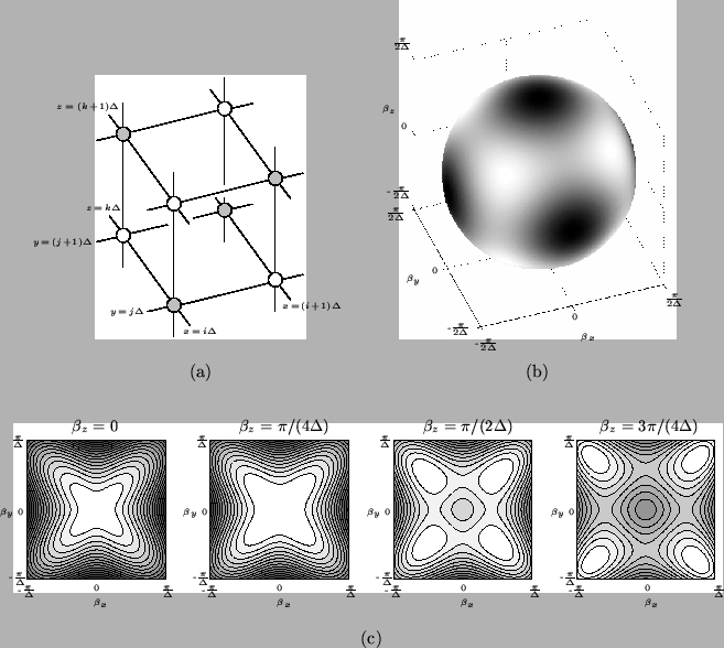
The tetrahedral scheme in (3+1)D [200] is somewhat similar to the hexagonal scheme in (2+1)D, in that the grid is divided evenly into two sets of points, at which updating is performed using ``mirror-image'' stencils. It is different, however, because grid points can easily be indexed with reference to a regular cubic lattice; the hexagonal scheme operates on a rectangular grid in stretched or transformed coordinates. In fact, a tetrahedral scheme can be obtained directly from an octahedral scheme simply by removing half of the grid points it employs; as such, any given grid point in the tetrahedral scheme has four nearest neighbors. As usual, we assume the nearest-neighbor grid spacing to be  . See Figure A.12(a) for a representation of the numerical grid.
As per the hexagonal scheme, we will view this as a vectorized scheme operating on two distinct sub grids, labeled 1 and 2 in Figure A.12(a). The two grid functions
 and
and
 are defined for integers
  ,
,  and
and  all even such that
  is also even.
 will be used to approximate a continuous function
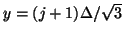
  at the point with coordinates
 ,
,
 and
and
 , and
, and
 approximates
  at coordinates
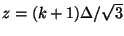
 ,
,
 and
and
 . The numerical scheme can then be written as
As for the hexagonal scheme, we may check consistency of this system with the wave equation by treating the grid functions as samples of continuous functions and and expanding (A.32) in terms of partial derivatives; both grid functions updated according to this scheme will approximate the solution to the wave equation on their respective grids.
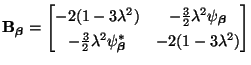
Determining the stability condition proceeds as in the hexagonal scheme; taking spatial Fourier transforms of (A.32) gives a vector spectral update equation of the form (A.10), with
 given by
with
is again Hermitian, and has eigenvalues
The stability condition can thus be written as
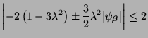 |
(A.34) |
 can be shown to take on a maximum of 4, and a minimum of 0, and it then follows that (A.33) will be satisfied if and only if
 , the same bound as obtained for the cubic rectilinear and octahedral schemes. The bound is the same as the bound for passivity of a tetrahedral mesh, as discussed in §4.7. We note that as for these other schemes, the grid permits a subdivision into mutually exclusive subschemes at this stability limit--see Figure A.12(a). By a simple comparison with the hexagonal scheme, we can obtain the four spectral amplification factors by
it is easy to see that parasitic modes (characterized by the amplification factors
 ) will be present in the tetrahedral scheme, due to the non-uniformity of updating on the numerical grid. The numerical dispersion characteristics of the dominant modes with amplification factors
 are shown in planar and spherical cross-sections in Figure A.12(b) and (c).
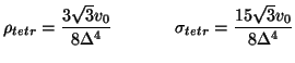
The computational and add densities of this scheme, in general, are
for
 , and
, and
at the stability limit
 .
.
Figure A.12:
The tetrahedral scheme (A.32)-- (a) numerical grid and connections, where grey/white coloring of points indicates a division into mutually exclusive subschemes at the stability bound. The scheme can be indexed similarly to the octahedral scheme (see Figure A.9). The two sub grids with mutually inverse orientations are labeled 1 and 2. (b)
 for the scheme at the stability bound
 , for a spherical surface with


 --the shading is normalized over the surface so that white corresponds to no dispersion error, and black to the maximum error over the surface (which is 6 per cent in this case). (c) Contour plots of
for various cross-sections of the space of spatial frequencies
; contours indicate successive deviations of 2 per cent from the ideal value of 1 which is obtained at spatial DC. Here we have only plotted spatial frequencies to
--the shading is normalized over the surface so that white corresponds to no dispersion error, and black to the maximum error over the surface (which is 6 per cent in this case). (c) Contour plots of
for various cross-sections of the space of spatial frequencies
; contours indicate successive deviations of 2 per cent from the ideal value of 1 which is obtained at spatial DC. Here we have only plotted spatial frequencies to
 ,
,
 , and
, and
 all less than
 .
.
 |
Next: Applications in Fluid Dynamics
Up: Finite Difference Schemes for
Previous: The (3+1)D Interpolated Rectilinear
Stefan Bilbao
2002-01-22