Next: Optimally direction-independent numerical dispersion
Up: Finite Difference Schemes for
Previous: The Rectilinear Scheme
The Interpolated Rectilinear Scheme
This scheme, like the standard rectilinear scheme, is defined over a grid with indices  and
and  , for points with
  and
and  . Updating, in this case, at a given point, requires access to values of the grid function at the previous time step at nearest-neighbor grid points to the north, east, west and south, as well as those to the north-east, north-west, south-east and south-west, which are more distant by a factor of
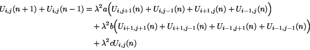
  . The scheme is referred to as ``interpolated'' in [157] because it is derived as an approximation to a hypothetical (and non-realizable) multi-directional difference scheme with minimally directionally-dependent numerical dispersion. (It is perhaps more useful to think of the scheme as interpolating between two rectilinear schemes operating on grids with a relative angle of 45 degrees.) The difference scheme will have the form
 |
(A.16) |
for constants  ,
,  and
and  which satisfy the constraints
 |
(A.17) |
for consistency with the wave equation. If  , we get the standard rectilinear scheme, and if
  , we get a rectilinear scheme operating on a grid of spacing
 , which is rotated by 45 degrees with respect to that of the standard scheme. This general form was put forth in [157], and the free parameter may be adjusted to give a less directionally-dependent numerical phase velocity; it may thus be used in conjunction with frequency-warping methods for reducing dispersion error. In general, the interpolated scheme cannot be decomposed into mutually exclusive subschemes.
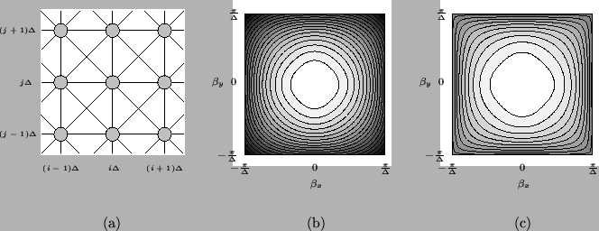
Figure A.2:
The interpolated rectilinear scheme (A.15)-- (a) numerical grid and connections for the interpolated rectilinear scheme (A.15); (b)
 of the scheme for
  at the ``passivity'' bound,
 ; (c)
for , at the stability bound, for
; (c)
for , at the stability bound, for
 .
.
 |
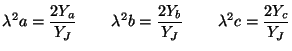
It is possible to examine the stability of this method as in the previous case. We again have an amplification polynomial equation of the form of (A.5), with
and thus
Note that
 is multilinear [3] in
 and
and
 , so that any extrema must occur at the corners of the region in the spatial frequency plane defined by
 , and
, and
 . Thus, we need evaluate
only for
. Thus, we need evaluate
only for 
![$ ^{T}=[\beta_{x}, \beta_{y}] = [0,0]$](img2902.png) ,
,
![$ [\pi/\Delta, 0]$](img2903.png) ,
,
![$ [0,\pi/\Delta]$](img2904.png) and
and
![$ [\pi/\Delta, \pi/\Delta]$](img2905.png) :
:
The global maximum of
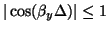
is non-positive (and thus condition (A.8) is satisfied) only if  . The global minimum of
, over this range of will then be
. The global minimum of
, over this range of will then be
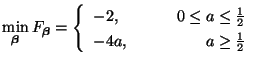
and the stability bound on  will be
 (for Von Neumann stability) (for Von Neumann stability) |
(A.18) |
It is interesting to look at the interpolated scheme from a waveguide mesh point of view (see Chapter 4 for details). At each grid point we will have a nine-port parallel scattering junction; four connections are made to neighboring points to the north, south, east and west, through a unit-delay bidirectional delay line of admittance  , four more connections are made to the points to the north-east, south-east, north-west and south-west using waveguides of admittance
  , and there will be a self-loop of admittance
  . If the junction voltage is written as
 , then the difference scheme corresponding to this waveguide mesh will be exactly (A.15), with
where the junction admittance  (assumed positive) will be given by
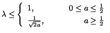
The passivity condition will then be a condition on the positivity of , and . From the previous discussion, we already require , so this ensures that
 . Requiring
 is equivalent to requiring
  ; from the first of constraints (A.16), this is true only for
  . Requiring
 is equivalent to requiring finally, from the second of constraints (A.16), that
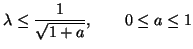 (for passivity) (for passivity) |
|
The difference between the constraints for stability from (A.17) and the passivity constraint above is striking; these bounds are graphed in Figure A.3.
Figure A.3:
Stability bounds for the interpolated rectilinear scheme, as a function of the free parameter . The solid line indicates the maximum value of for a given value of , and the dashed line the maximum value of allowed in a passive waveguide mesh implementation. Note that there is a passive realization only for
 .
.
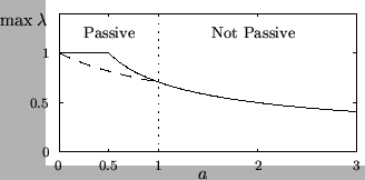 |
This is not the last time that we will find a discrepancy between Von Neumann stability of a scheme and passivity of the related mesh structure; it will come up again in the following section during a discussion of the triangular scheme, and in §A.3.3 when we look at the (3+1)D interpolated scheme. It is interesting to note that for a given value of , with
, the numerical dispersion properties can always be improved if we are willing to forgo passivity (and a mesh implementation). We have plotted the numerical phase velocities of this scheme for , at both the stability limit and the passivity limit in Figure A.2.
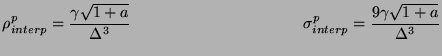
Finally, we mention that the computational and add densities for this scheme will be, in general,
over the range of  allowed by the stability constraint (A.17). For the scheme at the passivity bound (for
, with
allowed by the stability constraint (A.17). For the scheme at the passivity bound (for
, with  ), we have
We recall that for or  , at the stability limit, we again have the standard rectilinear scheme, for which a grid decomposition is possible; this was discussed in the previous section.
Subsections
Next: Optimally direction-independent numerical dispersion
Up: Finite Difference Schemes for
Previous: The Rectilinear Scheme
Stefan Bilbao
2002-01-22