The Rectilinear Scheme

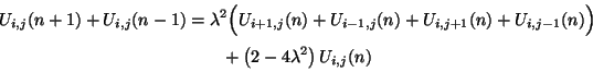
The finite difference scheme corresponding to a rectilinear mesh is obtained by applying centered differences to the wave equation, over a rectangular grid with indices $i$ and $j$ (which refer to points with spatial coordinates $x=i\Delta$ and $y=j\Delta$). The difference scheme, given originally as (4.53) is

$$\begin{split}U_{i,j}(n+1)+U_{i,j}(n-1) &= \lambda^{2}\Big(U_{... ...\ &\quad\quad+\left(2-4\lambda^{2}\right)U_{i,j}(n) \end{split}$$ (A.14)

and the amplification polynomial equation is of the form (A.5), with

$$B_{\mbox{{\scriptsize\boldmath$\beta$}}} = -2\Big(1+\lambda^{2}\left(\cos(\beta_{x}\Delta)+\cos(\beta_{y}\Delta)-2\right)\Big)$$

for $\beta$ $= [\beta_{x},\beta_{y}]^{T}$. From (A.7), we thus have

$$F_{\mbox{{\scriptsize\boldmath$\beta$}}} = \cos(\beta_{x}\Delta)+\cos(\beta_{y}\Delta)-2$$

and we have

$$\max_{\mbox{{\scriptsize\boldmath$\beta$}}}F_{\mbox{{\scriptsize\... ...ox{{\scriptsize\boldmath$\beta$}}}F_{\mbox{{\scriptsize\boldmath$\beta$}}} = -4$$

Condition (A.8) is thus satisfied, and condition (A.9) gives the bound

$$\lambda\leq\frac{1}{\!\!\sqrt{2}}$$

which implies that the amplification factor $\vert G_{\mbox{{\scriptsize\boldmath $\beta$}}, \pm}\vert = 1$ for such values of $\lambda$. Because $\lambda = \gamma/v_{0}$, this bound is the same as the bound for passivity of the associated mesh scheme, given in (4.63). The amplification factors, however, are distinct at all spatial frequencies only for $\lambda< 1/\sqrt{2}$. If $\lambda =1/\sqrt{2}$, then the factors are degenerate for $\beta_{x}=\beta_{y}=0$, and for $\beta_{x}=\beta_{y}= \pm\pi/\Delta$ and we are then in the situation discussed in §A.1.2 where linear growth of the solution may occur. This is an important special case, because it corresponds to the standard finite difference scheme for the rectilinear waveguide mesh (i.e., the realization without self-loops). The waveguide mesh implementation does not allow such growth at these frequencies.

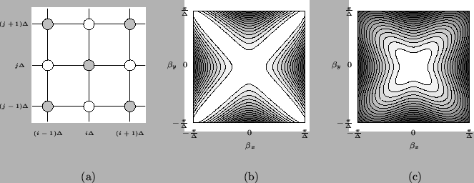
Figure A.1: The rectilinear scheme (A.13)-- (a) grid, of spacing $\Delta$, where grey/white coloring indicates a subgrid decomposition possible when $\lambda =1/\sqrt{2}$. (b) $v_{\mbox{{\scriptsize\boldmath$\beta$}}, phase}/\gamma$ for $\lambda =1/\sqrt{2}$. Contour lines are drawn, representing successive deviations of 2 per cent from the ideal value of 1 which is obtained at spatial DC. (c) $v_{\mbox{{\scriptsize\boldmath$\beta$}}, phase}/\gamma$ away from the stability bound, for $\lambda = 1/2$.

As far as assessing the computational requirements of the finite difference scheme, first consider the case $\lambda< 1/\sqrt{2}$. Five adds are required at each grid point in order to update. Given that $T = \Delta/v_{0}$, we can write the computational and add densities for the scheme as

$$\rho_{rect} = \frac{v_{0}}{\Delta^{3}}\hspace{0.3in}\sigma_{rect} = \frac{5v_{0}}{\Delta^{3}} \hspace{0.3in}v_{0}>\sqrt{2}\gamma$$

For $\lambda =1/\sqrt{2}$, however, scheme (A.13) simplifies to

$$U_{i,j}(n+1)+U_{i,j}(n-1) = \frac{1}{2}\Big(U_{i+1,j}(n)+U_{i-1,j}(n)+U_{i,j+1}(n)+U_{i,j-1}(n)\Big)$$ (A.15)

which may be operated on alternating grids, i.e., $U_{i,j}(n)$ need only be calculated for $i+j+n$ even (or odd). The computational and add densities, for $\lambda =1/\sqrt{2}$ are then

$$\rho_{rect}^{s} = \frac{v_{0}}{2\Delta^{3}}\hspace{0.3in}\sigma_{rect}^{s} = \frac{2v_{0}}{\Delta^{3}} \hspace{0.3in}v_{0}=\sqrt{2}\gamma$$

where we note that the reduced scheme (A.14) requires only four adds for updating at a given grid point; in addition, the multiplies by $1/2$ may be accomplished, in a fixed-point implementation, by simple bit-shifting operations. The increased efficiency of this scheme must be weighed against the danger of instability, and the fact that because grid density is reduced, the scheme is now applicable over a smaller range of spatial frequencies. The numerical phase velocities of the schemes, at the stability limit, and away from it, at $\lambda = 1/2$, are plotted in Figure A.1. It is interesting to note that away from the stability limit, the numerical dispersion is somewhat less directionally-dependent; this important factor may be useful from the point of view of frequency-warping techniques [157] which may be used to reduce numerical dispersion effects for schemes which are relatively directionally-independent. This idea has been discussed in the waveguide mesh context (where self-loops will be present) in [175].