Waveguide Network and the Wave Equation

Now consider the case in which $Y_{q,i}=Y$ is invariant over $i$ (and thus $q$, where again, $q$ stands for either $x^{+}$ or $x^{-}$). At all junctions, then, we have $Y_{J,i} = 2Y$. From (4.3.3) and (4.28), it is possible to obtain a finite difference scheme purely in terms of the junction voltages $U_{J,i}$. Beginning from (4.27), we have

$$U_{J,i}(n+1) = \frac{2}{Y_{J,i}}\left(Y_{x^{-},i}U_{x^{-},i}^{+}(n+1)+Y_{x^{+},i}U_{x^{+},i}^{+}(n+1)\right)\notag$$ (4.30)

$$= U_{x^{+},i-1}^{-}(n)+U_{x^{-},i+1}^{-}(n)\notag$$ (4.31)

$$= U_{J,i-1}(n)+U_{J,i+1}(n)-U_{x^{+},i-1}^{+}(n)- U_{x^{-},i+1}^{+}(n)\notag$$ (4.32)

$$= U_{J,i-1}(n)+U_{J,i+1}(n)- U_{x^{-},i}^{-}(n-1)-U_{x^{+},i}^{-}(n-1)\notag$$ (4.33)

$$= U_{J,i-1}(n)+U_{J,i+1}(n) -U_{J,i}(n-1)$$ (4.34)

This is identical to ( $\ref{magicdiff1d}$) if we replace $U_{J}$ by $U$. In this case of identical impedances in all the waveguides, there is no scattering, so the parallel junctions in Figure 4.8 reduce to simple ``throughs,'' and Figure 4.8 becomes Figure 4.9.

Figure 4.9: Simplified (1+1)D waveguide network.

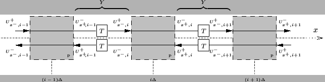Thus we have a discrete equivalent to the traveling wave solution to the wave equation, to be expected when the impedance does not vary spatially along the line. This particular case, which is trivial to implement (as a single many sample bidirectional delay line), has enormous applications to (1+1)D problems in homogeneous media, as were mentioned in §4.2.7. We also note that if the impedances do vary from one waveguide to the next, as in Figure 4.8, then we have a useful model of a system such as a tube with varying cross-sectional area or horn [66], a system whose impedance varies along its length, but whose wave speed remains constant. (In order to deal with local changes in the wave speed, we will have to introduce self-loops, which we will do shortly in §4.3.6.) This waveguide network is essentially equivalent to the Kelly-Lochbaum model used in speech synthesis [104], which we discussed in §1.1.1. It is interesting that linear predictive coding (LPC) [124], which is used to design filters to fit the spectrum of an analysis signal, essentially synthesizes a waveguide network like the one shown in Figure 4.8 (in effect it produces, as a by-product of the main calculation of direct-form filter coefficients, the reflection coefficients at the scattering junctions, from which impedances can then be deduced).