Music and Audio Applications of Digital Waveguides

Digital waveguide networks have been widely applied towards the synthesis of musical sound. Significant portions of many musical instruments can be simply modeled as nearly lossless uniform transmission lines: strings support transverse wave motion, and stiff strings and bars allow longitudinal and torsional motion as well; acoustic waves travel in the tubes that make up brass and wind instruments, organ pipes, as well as the human vocal tract, as we saw in §1.1.1. As such, there is a traveling wave decomposition of the motion in these systems.

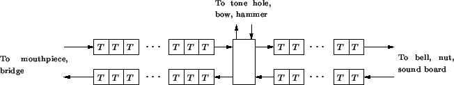
As we already mentioned in §4.2.3, a bidirectional delay line can be thought of as a discrete-time description of traveling wave propagation in a uniform transmission line. Thus a single waveguide, which is in itself no more than a pair of delay lines, can be used to model an uninterrupted stretch of a tube or string, without requiring any machine arithmetic. Scattering occurs only at the ends of the waveguide, and in fact, it is possible to use bidirectional delay lines to model wave propagation even in lossy [160] or dispersive [199] media by consolidating these effects at the terminations. If the length of the string or tube does not correspond to an integer number of delays at a given sample rate, then it is possible to employ fractional delay lines [114,195], which approximate non-integer delay lengths using all-pass (lossless) filters.

Figure 4.5: Typical digital waveguide configuration for musical sound synthesis.

A typical situation is shown in Figure 4.5. The string (or tube) is modeled as two bidirectional delay lines; at the extreme left and right, digital filters may be employed which model bridge terminations [164], horn bells and acoustic radiation [15,160], coupling with an instrument body or resonator such as a stringed instrument body [102], and, conceivably, coupling between different strings, and for a stiff string, even coupling between different types of motion (i.e. transverse, longitudinal and torsional). Excitation mechanisms (such as mouth pressure for a woodwind instrument [164] and lip pressure in brasses [15]) may be modeled as sources, are also used to terminate the waveguide; these may be linearly or nonlinearly coupled to the instrument body. If wave propagation is disturbed along the length of the tube or string, either by an excitation (such as a piano hammer [197] or bow [164]), or by an impedance change (due perhaps to a woodwind tone hole [160,194,196], or a change in the cross-sectional area of the vocal tract [30]), then these effects may be modeled at the junction between the two waveguides. In some situations, it may be necessary to employ a larger network of interconnected waveguides, as when the vocal tract is to be coupled with the nasal passageways. A full articulatory model of the human vocal tract has been built in this way to simulate the singing voice [30].

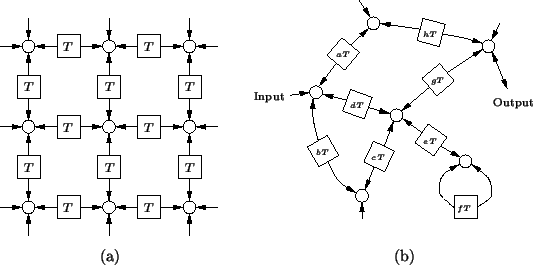
Digital waveguide networks have also been used to simulate wave motion in higher dimensions, in which case they are sometimes called waveguide meshes [198,200]; cases of particular interest have been (2+1)D meshes (see §1.1.2) used to simulate the vibration of a uniform membrane [67], and (3+1)D meshes used to model acoustic spaces [156]. Many different types of mesh have been proposed; they differ chiefly in their numerical dispersion properties [157], and we will analyze these forms in detail in Appendix A. A good deal of recent work has gone into the problem of correcting numerical dispersion by introducing terminating filters at the boundaries, and by using interpolation and frequency warping techniques [157]. A (2+1)D rectilinear mesh is shown in Figure 4.6(a). Unit-sample bidirectional delay lines (here represented by two-headed arrows) are connected to scattering junctions (white circles) located at the nodes of a rectangular lattice. Such a mesh has been used to model drum heads as well as gongs (where a nonlinear mesh termination has been applied) [197]. We mentioned in §1.1.2 that this mesh indeed solves the (2+1)D wave equation numerically [198]. We will elaborate on this idea extensively throughout the rest of the chapter.

Waveguide networks have also been used in a quasi-physical manner in order to effect artificial reverberation [163]. In this case, an unstructured network of waveguides of possibly time-varying impedance is used; such a network is shown in Figure 4.6(b), where the number of samples of delay in each waveguide (integers $a$ through $h$) may be different. Such networks are passive, so that signal energy injected into the network from a dry source signal will produce an output whose amplitude will gradually attenuate, with frequency-dependent decay times dependent on the delays and immittances of the various waveguides--some of the delay lengths can be interpreted as implementing ``early reflections.''[163]. Such networks provide a cheap and stable way of generating rich impulse responses. Generalizations of waveguide networks to feedback delay networks (FDNs) [149] and circulant delay networks [150] have also been explored, also with an eye towards applications in digital reverberation.

Figure 4.6: Other waveguide network configurations-- (a) a (2+1)D waveguide mesh, and (b) an unstructured network suitable for implementing artificial reverberation.

We will call these DWNs used for reverberation unstructured; by this we mean that the waveguides and scattering junctions are not necessarily arranged according to a regular grid in any coordinate system. Yet such a network is, by construction, passive. This contrasts sharply with the MDWD networks discussed in the previous chapter. In that case, discretization is performed through the use of a spectral mapping or integration rule; implicit in such an approach is that the algorithm operates on a regular grid in some system of coordinates (and the same will be true of the DWNs that are derived through an MDWD-like discretization procedure, as will be discussed in §4.10). The reason for this is that the DWN, as we have described it in this section, is essentially a large network of lumped elements, whereas the MDWD network is a multidimensional object. In certain cases (see §4.9), unstructured DWNs may come in handy.