Higher-order Accuracy

WDF-based numerical methods are, in general, second-order accurate in both the time step and the grid spacing. In all the schemes that have been examined in the literature, these quantities occur in a fixed ratio (usually written as $v_{0}$), so we can say that such schemes are accurate to second order in either one (or of any of the shift lengths in the new coordinates). A numerical approximation to a system of PDEs obtained using a MDWD network will converge to the solution to the model problem with a truncation error [176] proportional to the square of any of these spacings.

While this is true in general, in this section we would like to point out that it is indeed possible to devise MD circuit-based schemes which exhibit a higher-order spatial accuracy. Temporal accuracy, however, remains fixed at second-order; for this reason, such schemes must operate using a small time step; this limits their usefulness somewhat. Even more importantly, however, we note that the schemes we will develop here can be rewritten as very simple finite difference schemes of the form corresponding to digital waveguide networks (to be discussed in Chapter 4). We include this section merely to show that higher-order spatial accuracy is not incommensurate with MD-passivity, and to indicate a possible direction for future research.

Consider again the lossless source-free transmission line problem, defined by

$$\begin{eqnarray}l\frac{\partial i}{\partial t} +\frac{\partial u}... ...rac{\partial u}{\partial t} +\frac{\partial i}{\partial x} &=& 0 \end{eqnarray}$$ (3.96a)

(Losses and sources may be reintroduced at a later stage in these schemes without any difficulty.) Because higher-order spatially accurate explicit methods will require access to grid points other than nearest neighbors, we introduce the following coordinate transformation,

$${\bf H} = \begin{bmatrix}1&\!-1&2&\!-2&\hdots&q&-q\\ 1&1&1&1&\hdo... ... H}^{T}\begin{bmatrix}\frac{3}{q(2q+1)(q+1)}&0\\ 0&\frac{1}{2q}\\ \end{bmatrix}$$ (3.97)

for some positive integer $q$ (if $q=1$, then we get the coordinate transformation defined by (3.18), scaled by a constant factor). $2q$ will shortly be shown to be the order of spatial accuracy of the resulting difference scheme. As before, we have

$${\bf u} = {\bf V}^{-1}{\bf Ht}\hspace{1.0in}{\bf t} = {\bf H}^{-R}{\bf Vu}$$

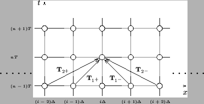
with ${\bf u} = [x, t]^{T}$, and ${\bf t} = [t_{1^{+}}, t_{1^{-}}, t_{2^{+}}, t_{2^{-}}, \hdots, t_{q^{+}}, t_{q^{-}}]^{T}$; the coordinate transformation defined by ${\bf H}$ thus describes an embedding of the (1+1)D problem in a $2q$-dimensional space. A uniform sampling of the new coordinates with spacings $T_{1^{+}} = T_{1^{-}} = \hdots = T_{q^{+}} = T_{q^{-}} = \Delta$ merely regenerates a uniform grid with spacing $\Delta$. 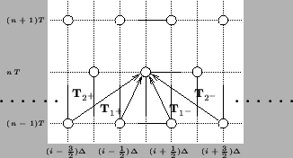The first two pairs of unit shifts are as shown in Figure 3.24.

Figure: Unit shifts in the coordinates defined by (3.94).

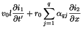
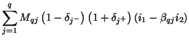
We now rewrite system (3.93) as

$$v_{0}l\frac{\partial i_{1}}{\partial t'} + r_{0}\sum_{j=1}^{q}\alpha_{qj}\frac{\partial i_{2}}{\partial x} =$$ 0

$$v_{0}cr_{0}^{2}\frac{\partial i_{2}}{\partial t'} + r_{0}\sum_{j=1}^{q}\alpha_{qj}\frac{\partial i_{1}}{\partial x} =$$ 0

where, as before, we have $i_{1} = i$, $i_{2} = u/r_{0}$ for some positive constant $r_{0}$, and $t^{'} = v_{0}t$. The $\alpha_{qj}$, $j=1,\hdots, q$, are constants which satisfy

$$\sum_{j=1}^{q}\alpha_{qj} = 1$$ (3.98)

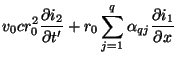
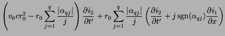
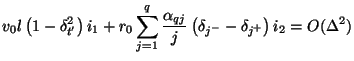
We may continue and write

$$\left(v_{0}l - r_{0}\sum_{j=1}^{q}\frac{\vert\alpha_{qj}\vert}{j}... ...{\partial t'}+j\,{\rm sgn}(\alpha_{qj})\frac{\partial i_{2}}{\partial x}\right) =$$ 0

$$\left(v_{0}cr_{0}^{2} - r_{0}\sum_{j=1}^{q}\frac{\vert\alpha_{qj}... ...{\partial t'}+j\,{\rm sgn}(\alpha_{qj})\frac{\partial i_{1}}{\partial x}\right) =$$ 0

Because, from (3.25), we have that

$$D_{j^{+}} \triangleq \frac{\partial}{\partial t_{j^{+}}} = \frac{... ...{\partial}{\partial t'}-j\frac{\partial}{\partial x}\hspace{0.3in}j=1,\hdots, q$$

we can immediately write

$$\begin{eqnarray}L_{1q}D_{t'}i_{1} + \sum_{j=1}^{q}M_{qj}\left(D_{... ...}+\beta_{qj}i_{1})+D_{j^{-}}(i_{2}-\beta_{qj}i_{1})\right) &=& 0 \end{eqnarray}$$ (3.99a)

with

$$L_{1q} = v_{0}l - r_{0}\sum_{j=1}^{q}\frac{\vert\alpha_{qj}\vert}... ..._{0}\vert\alpha_{qj}\vert}{2j}\hspace{0.3in}\beta_{qj} = {\rm sgn}(\alpha_{qj})$$ (3.100)

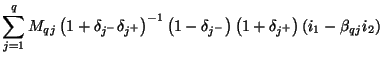
The system (3.96) can immediately be identified with an MDKC, as in Figure 3.25.

Figure: MDKC for the lossless source-free transmission line equations, according to the decomposition given by (3.96).

Each of the Jaumann two-ports can be discretized according to the trapezoid rule; as long as our choice of the constants $\alpha_{qj}$ satisfies the constraint (3.95) and $L_{1q}$ and $L_{2q}$ remain positive, the resulting MDWD network will be a second-order stable accurate approximation to system (3.93). Suppose, however, that we apply a different set of discretization rules, namely

$$\begin{eqnarray}D_{j^{+}} &\rightarrow& \frac{1}{\Delta}\left(1+\... ...\delta_{j^{-}}\right)\left(1+\delta_{j^{+}}\right)\hspace{0.3in} \end{eqnarray}$$ (3.101a)

for $j=1,\hdots, q$. Here, $\delta_{j^{+}}$ and $\delta_{j^{-}}$ are the shift operators in the directions $t_{j^{+}}$ and $t_{j^{-}}$ defined by

$$\delta_{j^{+}}e({\bf t}) = e({\bf t}-{\bf T}_{j^{+}}) \hspace{0.3in}\delta_{j^{-}}e({\bf t}) = e({\bf t}-{\bf T}_{j^{-}})$$

for a function $e({\bf t})$, where ${\bf T}_{j^{+}}$ and ${\bf T}_{j^{-}}$ are vectors of length $\Delta$ in directions $t_{j^{+}}$ and $t_{j^{-}}$ respectively (see Figure 3.24 for a graphical representation of these shifts on the computational grid). These rules correspond, in the linear shift-invariant case, to pairs of spectral mappings of the type mentioned briefly in §3.5.4, with shift lengths equal to $\Delta$; they are also MD-passivity preserving, and are in general second-order accurate [61]. To the scaled time derivative, we apply the trapezoid rule with a doubled time step $T' = 2\Delta$, as defined by

$$D_{t'}\rightarrow \frac{2}{T'}\left(1+\delta_{t'}^{2}\right)^{-1}... ...rac{1}{\Delta}\left(1+\delta_{t'}^{2}\right)^{-1}\left(1-\delta_{t'}^{2}\right)$$

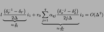
Equation (3.96a) then becomes

$$L_{1q}\left(1+\delta_{t'}^{2}\right)^{-1}\left(1-\delta_{t'}^{2}\right)i_{1}\!\! + \sum_{j=1}^{q}M_{qj}\left(1+\delta_{j^{-}}\delta_{j^{+}}\right)^{... ...\delta_{j^{+}}\right)\left(1+\delta_{j^{-}}\right)(i_{1}+\beta_{qj}i_{2})\notag$$ (3.102)

$$+ \sum_{j=1}^{q}M_{qj}\left(1+\delta_{j^{-}}\delta_{j^{+}}\right)^{... ...\delta_{j^{-}}\right)\left(1+\delta_{j^{+}}\right)(i_{1}-\beta_{qj}i_{2})\notag$$ (3.103)

$$= O(\Delta^{2})$$ (3.104)

Because, however, $\delta_{j^{+}}\delta_{j^{-}} = \delta_{t'}^{2}$ and our system is time-invariant, the operator $1+\delta_{j^{+}}\delta_{j^{-}}$ commutes with $L_{1q}$ and $M_{jq}$ and may be factored out of (3.99), giving

$$L_{1q}\left(1-\delta_{t'}^{2}\right)i_{1} + \sum_{j=1}^{q}M_{qj}\left(1-\delta_{j^{+}}\right)\left(1+\delta_{j^{-}}\right)(i_{1}+\beta_{qj}i_{2})\notag$$

$$+ \sum_{j=1}^{q}M_{qj}\left(1-\delta_{j^{-}}\right)\left(1+\delta_{j^{+}}\right)(i_{1}-\beta_{qj}i_{2})\notag$$

$$= O(\Delta^{2})$$

which can be further simplified to

$$v_{0}l\left(1-\delta_{t'}^{2}\right)i_{1}+r_{0}\sum_{j=1}^{q}\frac{\alpha_{qj}}{j}\left(\delta_{j^{-}}-\delta_{j^{+}}\right)i_{2} = O(\Delta^{2})$$

or, writing $\delta_{j^{-}} = \delta_{t'}\delta_{x}^{-j}$ and $\delta_{j^{+}} = \delta_{t'}\delta_{x}^{j}$ where $\delta_{x}$ is a simple shift in the $x$ direction of $\Delta$, as

$$l\underbrace{\frac{\left(\delta_{t'}^{-1}-\delta_{t'}\right)}{2\D... ...}\right)}{2j\Delta}}_{\approx \frac{\partial}{\partial x}}i_{2} = O(\Delta^{2})$$

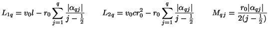
which is easily seen to be a simple difference approximation to (3.93a), The approximation is nominally second-order accurate in $\Delta$, but we have not as yet made any special choice of the $\alpha_{qj}$. This can be done via a conventional finite difference approach [176] in such a way as to yield a higher-order accurate approximation to the spatial derivative.

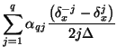
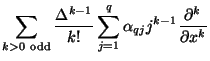
We can write, expanding the shift operators in Taylor series,

$$\sum_{j=1}^{q}\alpha_{qj}\frac{\left(\delta_{x}^{-j}-\delta_{x}^{j}\right)}{2j\Delta} = \sum_{k>0\,\,{\rm odd}}\frac{\Delta^{k-1}}{k!}\sum_{j=1}^{q}\alpha_{qj}j^{k-1}\frac{\partial^{k}}{\partial x^{k}}$$ (3.105)

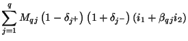
There are $q$ degrees of freedom, corresponding to the parameters $\alpha_{qj}$, $j=1,\hdots, q$. We require, from (3.95) that the coefficient of the first derivative on the right-hand side of (3.100) equal one. We may then additionally require that the other coefficients, for $k=3, \hdots, 2q+1$ be zero; the resulting difference approximation will then be accurate to order $2q$. This yields the linear system

$${\bf C} \mbox{\boldmath$\alpha$} _{q} = {\bf e}_{q}$$ (3.106)

where ${\bf C}$ is a $q\times q$ matrix with $[{\bf C}_{ij}] = j^{2(i-1)}$, $\alpha$ $_{q} = [\alpha_{q1},\hdots,\alpha_{qq}]^{T}$, and ${\bf e}_{q}$ is a $q\times 1$ vector whose first entry is one, and whose others are zero. ${\bf C}$ is always full rank, so there is a unique solution for any $q$. The same $\alpha$$_{q}$ will also give a higher-order approximation to (3.93b), and thus system (3.93) will be approximated to higher-order accuracy as a whole. For a fourth-order approximation, for example, we obtain $\alpha$ $_{2}= [4/3,-1/3]^{T}$, and for a sixth-order approximation, we get $\alpha$ $_{3}= [3/2, -3/5, 1/10]^{T}$. These values completely determine the MDKC pictured in Figure 3.25.

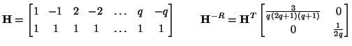
The passivity requirement is, as before, a condition on the positivity of $L_{1q}$ and $L_{2q}$. Choosing $r_{0} = \sqrt{l_{min}/c_{min}}$ gives

$$v_{0} \geq \frac{3}{2\sqrt{l_{min}c_{min}}}$$

$$v_{0} \geq \frac{11}{6\sqrt{l_{min}c_{min}}}$$

It is interesting to note that in the constant-coefficient case, this bound is distinct from the stability bound obtained from Von Neumann analysis (see Appendix A) applied to the same difference method. For example, for the fourth-order accurate scheme defined by $\alpha$$_{2}$, the stability bound is $v_{0}\geq 1.37 \gamma$, with $\gamma = 1/\sqrt{lc}$; there is thus a range of values of $v_{0}$ for which the scheme will be stable, but not MD-passive. We will comment extensively on the distinction between passive and stable methods in Appendix A.

It is also of interest to define a similar scheme with respect to the coordinate transformation defined by

$${\bf H} = \begin{bmatrix}\frac{1}{2}&\!-\frac{1}{2}&\frac{3}{2}&\... ...2}&\hdots&\frac{2q-1}{2}&\!-\frac{2q-1}{2}\\ 1&1&1&1&\hdots&1&1\\ \end{bmatrix}$$ (3.107)

Keeping the same notation for the new coordinates, the shifts are as shown in Figure 3.26; now we have a grid ideal for a staggered or interleaved algorithm, with alternating grid points at alternating time steps.

Figure: Unit shifts in the coordinates defined by (3.102).

For this coordinate system, we follow through a development very similar to that in the previous pages. We again have an MD circuit representation as in Figure 3.25, where now we have

$$L_{1q} = v_{0}l-r_{0}\sum_{j=1}^{q}\frac{\vert\alpha_{qj}\vert}{j... ...}{2}}\hspace{0.3in}M_{qj} = \frac{r_{0}\vert\alpha_{qj}\vert}{2(j-\frac{1}{2})}$$

for some set of $\alpha_{qj}$, $j=1,\hdots, q$ which sum to unity. The symbols $D_{j^{+}}$ and $D_{j^{-}}$ in the figure now refer to directional derivatives in the coordinate directions defined by (3.102). For higher-order accuracy, constraint equation (3.101) will apply, now with $[{\bf C}_{ij}] = (j-1/2)^{2(i-1)}$. For fourth-order accuracy, we obtain $\alpha$ $_{2}= [9/8, -1/8]^{T}$, and for a sixth-order approximation, we get $\alpha$ $_{3}\approx [1.179, -0.195, 0.0234]^{T}$.

Because here we are using an alternative discretization rule, the resulting MDWD networks are more appropriately discussed in the context of digital waveguide networks (which are the subject of the next chapter). We will return briefly to waveguide network representations of these higher-order accurate methods in §4.10.5.