Next: The Waveguide Mesh
Up: The (2+1)D Parallel-plate System
Previous: The (2+1)D Parallel-plate System
The set of PDEs describing a lossless, source-free parallel-plate transmission line in (2+1)D is a direct generalization of system (4.17):
 |
(4.60a) |
Now
 and
and
 are the components of the current density vector in the
  and
and  directions, respectively, and
  is the voltage between the plates.
  and
and  , both assumed positive everywhere, are the inductance and capacitance per unit length.
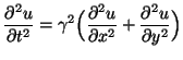
If we assume that  and
and  are constant, then as in the (1+1)D case, the set of equations can be reduced to a single second order equation in the voltage alone:
 |
(4.61) |
and again, the wave speed  is given by
The centered difference scheme for system (4.49) also generalizes simply. Define grid functions
 ,
,
 and
and
 which run over half-integer values of
  ,
,  , and
, and  , i.e.,
We will furthermore assume that the spatial step in the direction and the direction are the same and equal to  . As before, the time step will be
  .
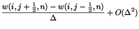
We can use the approximations (4.19), as well as an approximation to the derivative in the direction,
.
We can use the approximations (4.19), as well as an approximation to the derivative in the direction,
where  stands for either of
  or
or  .
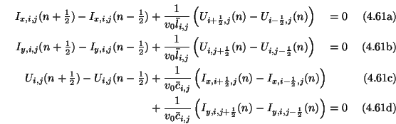
We obtain the difference scheme
.
We obtain the difference scheme
where we have written
and
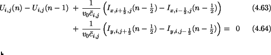
As in the (1+1)D case, it is possible to subdivide the calculation scheme (4.51) into smaller, mutually exclusive subschemes. Using a decimated grid for the variable coefficient difference scheme amounts to rewriting scheme (4.51) as
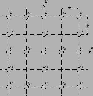
where we now compute solutions for , and integer. The interleaved grid is shown in Figure 4.18; a grey (white) dot at a grid location indicates that the adjacent named variable is to be calculated at times which are even (odd) multiples of . This interleaved form was originally put forth by Yee [214] in the context of electromagnetic field problems, and forms the basis of the widely used finite-difference time domain (FDTD) family of difference methods [184], which were discussed briefly in §4.1. If system (4.52) is rewritten as a TE or TM system, the interleaved arrangement of the field components also has an interesting physical interpretation as a discrete counterpart to the integral form of Ampere's and Faraday's Laws [184]. This result also extends easily to the discretization of Maxwell's equations in (3+1)D [214]; see §4.10.6 for more details.
Figure 4.18:
Interleaved computational grid for the (2+1)D parallel-plate system.
 |
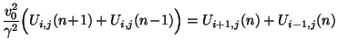
The (2+1)D analogue of (4.23), which holds in the case where and are constant, is
The magic time step will now be
and (4.53) simplifies to
 |
(4.66) |
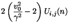
As in (1+1)D, when we are solving the wave equation by centered differences at the magic time step (or at CFL), the calculation further decomposes into two independent calculations; we need only update
for  even (or odd). We will examine this interesting decomposition property in detail in Appendix A.
Next: The Waveguide Mesh
Up: The (2+1)D Parallel-plate System
Previous: The (2+1)D Parallel-plate System
Stefan Bilbao
2002-01-22