Vector Wave Variables

It is straightforward to extend wave digital filtering principles to the vector case (this has been outlined in [131]; the same idea has apeared in the context of digital waveguide networks in [166,169]). For a $q$-component vector one-port element with voltage ${\bf v} = [v_{1}, \hdots, v_{q}]^{T}$ and current ${\bf i} = [i_{1}, \hdots, i_{q}]^{T}$, it is posible to define wave variables ${\bf a}$ and ${\bf b}$ by

$$\begin{eqnarray}{\bf a} &=& {\bf v} + {\bf Ri}\\ {\bf b} &=& {\bf v} - {\bf Ri} \end{eqnarray}$$ (2.43a)

for a $q\times q$ symmetric positive definite matrix ${\bf R}$; power-normalized quantities may be defined by

$$\begin{eqnarray}\underline{{\bf a}} &=& \frac{1}{2}\left({\bf R}^... ...\frac{1}{2}\left({\bf R}^{-T/2}{\bf v} - {\bf R}^{1/2}{i}\right) \end{eqnarray}$$ (2.44a)

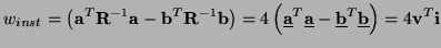
where ${\bf R}^{1/2}$ is some right square root of ${\bf R}$, and ${\bf R}^{T/2}$ is its transpose. The power absorbed by the vector one-port will be

$$w_{inst} = \left({\bf a}^{T}{\bf R}^{-1}{\bf a}-{\bf b}^{T}{\bf R... ...\bf a}}-\underline{{\bf b}}^{T}\underline{{\bf b}}\right) = 4{\bf v}^{T}{\bf i}$$ (2.45)

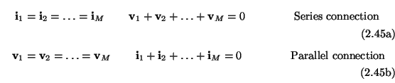
Kirchoff's Laws, for a series or parallel connection of $M$ $q$-component vector elements with voltages ${\bf v}_{j}$ and ${\bf i}_{j}$, $j=1,\hdots,M$ can be written as

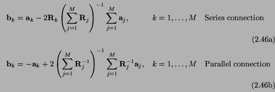
and the resulting scattering equations will be

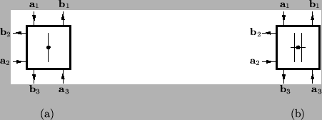
in terms of the wave variables ${\bf a}_{k}$, ${\bf b}_{k}$ defined as per (2.43) and the port resistance matrices ${\bf R}_{k}$, $k=1,\hdots,M$. These are the defining equations of a vector adaptor; their schematics are essentially the same as those of Figure 2.12, except that they are drawn in bold--see Figure 2.14. As before, we use the same representation for power-normalized waves.

Figure 2.14: Three-port vector adaptors-- (a) a vector series adaptor and (b) a vector parallel adaptor.