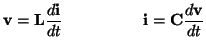
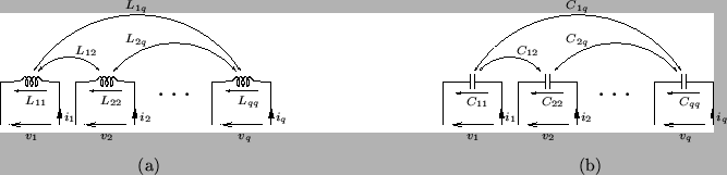
We show an inductive coupling of ![]() loops in Figure 2.15(a); self-inductances are indicated by directed arrows, accompanied by an inductance
loops in Figure 2.15(a); self-inductances are indicated by directed arrows, accompanied by an inductance ![]() ,
,
![]() (these are the diagonal elements of
(these are the diagonal elements of ![]() ), and a mutual inductance between loops
), and a mutual inductance between loops ![]() and
and ![]() ,
, ![]() is represented by an arrow and the associated inductance
is represented by an arrow and the associated inductance ![]() (which is the
(which is the ![]() th or
th or ![]() th element of
th element of ![]() , and is not constrained to be positive). A coupled capacitance is shown in Figure 2.15(b).
, and is not constrained to be positive). A coupled capacitance is shown in Figure 2.15(b).
A coupled inductance can be discretized through the use of the trapezoid rule applied directly to the vector equations of (2.48); in terms of wave variables defined by (2.43), we get
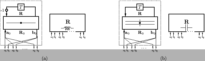
In practice, if a coupled inductance (or capacitance) appears in a circuit which is to be discretized using WDFs, we may treat it as a ![]() -vector two-port made up of a series (or parallel) junction terminated on a vector wave digital inductor (or capacitor) of port resistance
-vector two-port made up of a series (or parallel) junction terminated on a vector wave digital inductor (or capacitor) of port resistance
![]() (or
(or
![]() ). See Figure 2.16 for the signal flow diagrams for these objects and the simplified representations that we will use. The port resistance at the opposing port will in general be diagonal, so that the vector wave variables entering and leaving the junction may be decomposed into scalar wave variables; this diagonal port resistance will be determined by the rest of the network to which the
). See Figure 2.16 for the signal flow diagrams for these objects and the simplified representations that we will use. The port resistance at the opposing port will in general be diagonal, so that the vector wave variables entering and leaving the junction may be decomposed into scalar wave variables; this diagonal port resistance will be determined by the rest of the network to which the ![]() -vector two-port is connected. See §4.2.6 for more information on this decomposition in the DWN context; we will return to vector/scalar connections in Chapter 5. We note that in the representations in Figure 2.16, we have not explicitly indicated the order in which the
-vector two-port is connected. See §4.2.6 for more information on this decomposition in the DWN context; we will return to vector/scalar connections in Chapter 5. We note that in the representations in Figure 2.16, we have not explicitly indicated the order in which the ![]() scalar incoming and outgoing vectors should be ``packed'' and ``unpacked'' from the vector wave variables at the lower ports of the vector junctions. In the applications in Chapter 5, for a given coupled inductance (say), self-inductances will all be identical, as will all mutual inductances; thus any ordering will do, as long as the
scalar incoming and outgoing vectors should be ``packed'' and ``unpacked'' from the vector wave variables at the lower ports of the vector junctions. In the applications in Chapter 5, for a given coupled inductance (say), self-inductances will all be identical, as will all mutual inductances; thus any ordering will do, as long as the ![]() th elements of both
th elements of both ![]() and
and ![]() correspond to wave variables at the
correspond to wave variables at the ![]() th scalar port.
th scalar port.
 |