- ...
email1.1
- jos at ccrma
.
.
.
.
.
.
.
.
.
.
.
.
.
.
.
.
.
.
.
.
.
.
.
.
.
.
.
.
.
.
- ... FFT2.1
- ``Fast Fourier
Transform'' -- fast algorithms for implementing the Discrete Fourier
Transform (DFT) [264].
.
.
.
.
.
.
.
.
.
.
.
.
.
.
.
.
.
.
.
.
.
.
.
.
.
.
.
.
.
.
- ...
(DTFT).3.1
- In practical situations we can only deal with
finite-duration signals, so really we always use the Discrete Fourier
Transform (DFT) [264]. Moreover, the DFT is typically
implemented using the split-radix Cooley-Tukey Fast Fourier Transform
(FFT), which requires the DFT length to be a power of 2. Thus, in
practice, we use an FFT, while for theoretical studies, the DTFT is
preferred.
.
.
.
.
.
.
.
.
.
.
.
.
.
.
.
.
.
.
.
.
.
.
.
.
.
.
.
.
.
.
- ...MDFT.3.2
- http://ccrma.stanford.edu/~jos/mdft/Fourier_Theorems_DFT.html
.
.
.
.
.
.
.
.
.
.
.
.
.
.
.
.
.
.
.
.
.
.
.
.
.
.
.
.
.
.
- ... variable,3.3
- The symbol ``
 '' means ``is
defined as'' or ``equals by definition.'' In conformity with typical
signal-processing literature, most of this chapter
uses normalized frequency, i.e., the sampling rate equals
'' means ``is
defined as'' or ``equals by definition.'' In conformity with typical
signal-processing literature, most of this chapter
uses normalized frequency, i.e., the sampling rate equals
 sample per second.
.
.
.
.
.
.
.
.
.
.
.
.
.
.
.
.
.
.
.
.
.
.
.
.
.
.
.
.
.
.
- ...MDFT.3.4
- http://ccrma.stanford.edu/~jos/mdft/Fourier_Theorems.html
.
.
.
.
.
.
.
.
.
.
.
.
.
.
.
.
.
.
.
.
.
.
.
.
.
.
.
.
.
.
- ... states3.5
- Our
notational convention is that the first subscripts of an operator such
as
 are its parameters, as in
 , and the last
subscript selects a particular sample of output, as in
, and the last
subscript selects a particular sample of output, as in
 . If the last subscript is omitted, it ``returns''
an entire signal. Thus,
is a scalar while
is an entire signal defined over the integers. We
also may use
. If the last subscript is omitted, it ``returns''
an entire signal. Thus,
is a scalar while
is an entire signal defined over the integers. We
also may use  to denote all values of some index, e.g.,
 .
.
.
.
.
.
.
.
.
.
.
.
.
.
.
.
.
.
.
.
.
.
.
.
.
.
.
.
.
.
.
.
- ... cases.3.6
- For
definitions of the DFT, DTFT, FT, and FS, see Table 2.1
.
.
.
.
.
.
.
.
.
.
.
.
.
.
.
.
.
.
.
.
.
.
.
.
.
.
.
.
.
.
- ...3.7
- If the sampling density is not sufficiently high, there will
be aliasing (wrap-around) in the time domain. DTFT sampling
in the frequency domain is an exact Fourier dual of ordinary
sampling in the time domain.
.
.
.
.
.
.
.
.
.
.
.
.
.
.
.
.
.
.
.
.
.
.
.
.
.
.
.
.
.
.
- ...MDFT:3.8
- http://ccrma.stanford.edu/~jos/mdft/Zero_Padding.html
.
.
.
.
.
.
.
.
.
.
.
.
.
.
.
.
.
.
.
.
.
.
.
.
.
.
.
.
.
.
- ...
practice.3.9
- Nevertheless, as discussed in [266],
a perceptually exact
band-limited interpolation can be implemented at a reasonable cost in
the time domain, provided some amount of
oversampling is used. Oversampling in the time domain provides
a guard band in the frequency domain, which enables the
interpolation kernel to meet perceptually ideal specifications at a
much smaller length [270].
.
.
.
.
.
.
.
.
.
.
.
.
.
.
.
.
.
.
.
.
.
.
.
.
.
.
.
.
.
.
- ...spectsamps.3.10
- In particular, zero-padding does not increase the resolution
of an FFT. This is a surprisingly common point of misunderstanding
(or sometimes just mislabeling).
.
.
.
.
.
.
.
.
.
.
.
.
.
.
.
.
.
.
.
.
.
.
.
.
.
.
.
.
.
.
- ... work.3.11
- One could say the
Blackman window is well matched to ``analog synthesizer quality''
levels, where a 60 dB signal-to-noise ratio is common.
.
.
.
.
.
.
.
.
.
.
.
.
.
.
.
.
.
.
.
.
.
.
.
.
.
.
.
.
.
.
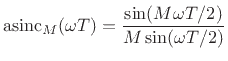
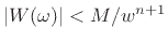
- ...
function|textbf:4.1
- Note that writing
 to denote the aliased
sinc function is not standard practice in signal processing--consider
it proposed notation.
to denote the aliased
sinc function is not standard practice in signal processing--consider
it proposed notation.
.
.
.
.
.
.
.
.
.
.
.
.
.
.
.
.
.
.
.
.
.
.
.
.
.
.
.
.
.
.
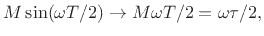
- ....4.2
- In more detail, start with the ``physical'' definition of
:
 |
(4.9) |
Now replace  by
by  in the numerator. Take the limit as
  goes to zero, with
remaining fixed, so that
goes to zero, with
remaining fixed, so that  goes to
infinity (maintaining the relation
goes to
infinity (maintaining the relation
 ). When
gets very
small, the denominator becomes
). When
gets very
small, the denominator becomes
 |
(4.10) |
which completes the proof.
.
.
.
.
.
.
.
.
.
.
.
.
.
.
.
.
.
.
.
.
.
.
.
.
.
.
.
.
.
.
- ... crossings.4.3
 is the
radian-frequency sampling interval for a length
DFT. Using
to denote the sampling interval along
is the
radian-frequency sampling interval for a length
DFT. Using
to denote the sampling interval along  is analogous
to using
to denote the sampling interval along time
is analogous
to using
to denote the sampling interval along time  -- hence
the choice of symbol
-- hence
the choice of symbol  .
.
.
.
.
.
.
.
.
.
.
.
.
.
.
.
.
.
.
.
.
.
.
.
.
.
.
.
.
.
.
.
- ...Harris78.4.4
- The Hamming window can also be derived as a
special case of windows having a maximized main-lobe peak
 over
all windows of the same energy and prescribed first zero-crossings
about the main lobe
[202, p. 239,403].
over
all windows of the same energy and prescribed first zero-crossings
about the main lobe
[202, p. 239,403].
.
.
.
.
.
.
.
.
.
.
.
.
.
.
.
.
.
.
.
.
.
.
.
.
.
.
.
.
.
.
- ...Harris78.4.5
- Note that the
 dB figure is
for large window-length
. For small window lengths, the side-lobe
levels increase. This phenomenon can be understood in terms of
aliasing of the side-lobes of the continuous Hamming window which must
be sampled to obtain a discrete-time window.
dB figure is
for large window-length
. For small window lengths, the side-lobe
levels increase. This phenomenon can be understood in terms of
aliasing of the side-lobes of the continuous Hamming window which must
be sampled to obtain a discrete-time window.
.
.
.
.
.
.
.
.
.
.
.
.
.
.
.
.
.
.
.
.
.
.
.
.
.
.
.
.
.
.
- ... dB,4.6
- For larger
window-length
, more than
 dB side-lobe suppression can be
achieved, such as the
value cited in [101].
dB side-lobe suppression can be
achieved, such as the
value cited in [101].
.
.
.
.
.
.
.
.
.
.
.
.
.
.
.
.
.
.
.
.
.
.
.
.
.
.
.
.
.
.
- ... Hann4.7
- The precise side-lobe level is dependent on window
length
, but
to
 dB is typical for the Hamming
window.
dB is typical for the Hamming
window.
.
.
.
.
.
.
.
.
.
.
.
.
.
.
.
.
.
.
.
.
.
.
.
.
.
.
.
.
.
.
- ...Papoulis.4.8
- The proof that
(3.36) is maximized appears on p. 210 of [202].
.
.
.
.
.
.
.
.
.
.
.
.
.
.
.
.
.
.
.
.
.
.
.
.
.
.
.
.
.
.
- ....4.9
- From a
linear algebra point of view, consider the sinc kernel as
corresponding to a Toeplitz Hermitian matrix. It is well known
that Hermitian matrices have real eigenvalues and orthogonal
eigenvectors. Also, multiplication by a Toeplitz matrix corresponds
to convolution (in this case, a non-causal convolution.)
.
.
.
.
.
.
.
.
.
.
.
.
.
.
.
.
.
.
.
.
.
.
.
.
.
.
.
.
.
.
- ...
Box4.10
- For Octave, the original version by Eric Breitenberger is
still available on the Web, as of this writing, at
http://pangea.stanford.edu/Oceans/GES290/Breitenberger-SSAMatlab/mtm/.
Note, however, that the calling arguments after the first two are
differently defined. A simple version written by the author appears
in §F.1.2.
.
.
.
.
.
.
.
.
.
.
.
.
.
.
.
.
.
.
.
.
.
.
.
.
.
.
.
.
.
.
- ... by4.11
- For small
and/or
 , the closed-form transform diverges from the DTFT of the
discrete-time Kaiser window due to aliasing.
, the closed-form transform diverges from the DTFT of the
discrete-time Kaiser window due to aliasing.
.
.
.
.
.
.
.
.
.
.
.
.
.
.
.
.
.
.
.
.
.
.
.
.
.
.
.
.
.
.
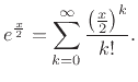
- ... kind:4.12
- The Maclaurin series for
 can be obtained as
the term-by-term square of that for
can be obtained as
the term-by-term square of that for  , since
 |
(4.41) |
.
.
.
.
.
.
.
.
.
.
.
.
.
.
.
.
.
.
.
.
.
.
.
.
.
.
.
.
.
.
- ... radians-per-second).4.13
- In
[101],
 is described as half of
the time-bandwidth product, which in turn is not defined. Factors of
2 often come and go because, e.g., the frequency band
is described as half of
the time-bandwidth product, which in turn is not defined. Factors of
2 often come and go because, e.g., the frequency band
![$ [-\omega_c,\omega_c]$](img468.png) is often considered a bandwidth of
is often considered a bandwidth of  (neglecting negative frequencies).
.
.
.
.
.
.
.
.
.
.
.
.
.
.
.
.
.
.
.
.
.
.
.
.
.
.
.
.
.
.
- ....4.14
- The causal version may be
computed as the inverse DFT of
 .
.
.
.
.
.
.
.
.
.
.
.
.
.
.
.
.
.
.
.
.
.
.
.
.
.
.
.
.
.
.
.
- ...
itself.4.15
- The not-so-smooth function
 also
transforms to itself
[150, p. 47]. Also, a periodic impulse train transforms
to an impulse train with reciprocal spacing of the impulses
(see §B.14). Finally, as discussed at
http://www.dsprelated.com/showarticle/45.php,
if
also
transforms to itself
[150, p. 47]. Also, a periodic impulse train transforms
to an impulse train with reciprocal spacing of the impulses
(see §B.14). Finally, as discussed at
http://www.dsprelated.com/showarticle/45.php,
if  is real and even, then
 is its own transform
under the normalized Fourier transform. (The normalized Fourier
transform is the usual Fourier transform divided by
is its own transform
under the normalized Fourier transform. (The normalized Fourier
transform is the usual Fourier transform divided by
 ,
which results in the inverse transform having the same scale factor.)
That is,
,
which results in the inverse transform having the same scale factor.)
That is,
 .
We used the fact that if
is real and even, then so is
.
We used the fact that if
is real and even, then so is
 . (This is shown for the DTFT case in §2.3.3,
and the proof is analogous in the continuous-time case.) Note that
for
. (This is shown for the DTFT case in §2.3.3,
and the proof is analogous in the continuous-time case.) Note that
for  to be smooth (differentiable of all orders), it cannot be
bandlimited in either time or frequency.
to be smooth (differentiable of all orders), it cannot be
bandlimited in either time or frequency.
.
.
.
.
.
.
.
.
.
.
.
.
.
.
.
.
.
.
.
.
.
.
.
.
.
.
.
.
.
.
- ... design.4.16
- A spectrum-analysis window
may be regarded as an FIR lowpass filter having an extremely narrow
pass-band.
.
.
.
.
.
.
.
.
.
.
.
.
.
.
.
.
.
.
.
.
.
.
.
.
.
.
.
.
.
.
- ...
CPUs5.1
- In recent years, Graphics Processing Units (GPUs) have
been used increasingly for high-performance general-purpose digital
signal processing [242]. For example, the NVIDIA
CUDA development environment allows harnessing of many parallel
threads of execution in a GPU (typically on a graphics card or
chip-set in a personal computer) from a C program using GPU-related
library extensions. Due to the massive parallelism available in a GPU,
FFT convolution becomes competitive with time-domain convolution only
at much longer lengths (in the thousands) [242]. In a
CPU (one processor), FFT methods typically win out for convolution
lengths greater than 100 or so (see §8.1.4 for some
details).
.
.
.
.
.
.
.
.
.
.
.
.
.
.
.
.
.
.
.
.
.
.
.
.
.
.
.
.
.
.
- ... frequencies.5.2
- In this book, unless
specified otherwise, all frequencies are normalized by the
sampling rate. Thus,
 is physically ``cycles per
sample.''
is physically ``cycles per
sample.''
.
.
.
.
.
.
.
.
.
.
.
.
.
.
.
.
.
.
.
.
.
.
.
.
.
.
.
.
.
.
- ...optfirlp.5.3
- In fact,
optimal window design is a special case of optimal FIR lowpass design
in which the desired pass-band width is nearly zero, as we will see.
.
.
.
.
.
.
.
.
.
.
.
.
.
.
.
.
.
.
.
.
.
.
.
.
.
.
.
.
.
.
- ...
audible.5.4
- A 0.1 dB pass-band ripple results in a normally
inaudible amplitude error, while a -60 dB stop-band ripple can be
quite audible if the pass-band is relatively quiet and high signal
energy appears in the stop-band.
.
.
.
.
.
.
.
.
.
.
.
.
.
.
.
.
.
.
.
.
.
.
.
.
.
.
.
.
.
.
- ... frequency)5.5
- It is a
common matlab convention to specify normalized frequencies between
0 and 1 such that 1 corresponds to half the sampling rate,
instead of the sampling rate. Thus, one-fourth the sampling rate
(
 ) is specified as
  in matlab. In this
book, outside of Matlab function arguments, normalized frequency
in matlab. In this
book, outside of Matlab function arguments, normalized frequency
 is always the sampling rate.
.
.
.
.
.
.
.
.
.
.
.
.
.
.
.
.
.
.
.
.
.
.
.
.
.
.
.
.
.
.
- ....5.6
- As a result of the implicit equal weighting, the
stop-band ripple at
 dB means that the pass-band ripple
is below 0.007 dB, which is overkill for typical audio applications.
This pass-band ripple can be enlarged in exchange for improved
stop-band ripple or a narrower transition band or both. This is done
by specifying a larger weighting on the stop-band ripple--see the
help page for firpm for details.
dB means that the pass-band ripple
is below 0.007 dB, which is overkill for typical audio applications.
This pass-band ripple can be enlarged in exchange for improved
stop-band ripple or a narrower transition band or both. This is done
by specifying a larger weighting on the stop-band ripple--see the
help page for firpm for details.
.
.
.
.
.
.
.
.
.
.
.
.
.
.
.
.
.
.
.
.
.
.
.
.
.
.
.
.
.
.
- ... design5.7
- Recall that window
design can be formulated as FIR lowpass-filter design with a
zero-with (or nearly zero-width) pass-band.
.
.
.
.
.
.
.
.
.
.
.
.
.
.
.
.
.
.
.
.
.
.
.
.
.
.
.
.
.
.
- ... ``tight''.5.8
- Our choice came from
 as used in [228].
.
.
.
.
.
.
.
.
.
.
.
.
.
.
.
.
.
.
.
.
.
.
.
.
.
.
.
.
.
.
- ...RabinerAndGold.5.9
- Show this as an exercise. [Hint: Recall
the stretch theorem (§2.3.11).]
.
.
.
.
.
.
.
.
.
.
.
.
.
.
.
.
.
.
.
.
.
.
.
.
.
.
.
.
.
.
- ... response.5.10
- It is effective in
practice to try doubling the FFT size to see if it appreciably
changes the designed filter--it should not.
.
.
.
.
.
.
.
.
.
.
.
.
.
.
.
.
.
.
.
.
.
.
.
.
.
.
.
.
.
.
- ... consequences.5.11
- However, consider an
FM signal in which a sinusoid is sweeping back and forth in the
pass-band. In that case, the pass-band-ripple generates AM
sidebands, so a spec more like that in the stop-band may be called
for. Here, we allow the pass-band ripple to be 10 times the
stop-band ripple, which is a reasonable compromise.
.
.
.
.
.
.
.
.
.
.
.
.
.
.
.
.
.
.
.
.
.
.
.
.
.
.
.
.
.
.
- ... gains.5.12
- While cubic splines are maximally
smooth in a precise physical sense, they are not band-limited, so
one can do better by using band-limited interpolation of the
desired frequency-response points. (In this situation,
``band-limited'' equals ``time-limited,'' which is exactly what we
are going for in an FIR filter design.)
.
.
.
.
.
.
.
.
.
.
.
.
.
.
.
.
.
.
.
.
.
.
.
.
.
.
.
.
.
.
- ...
Octave).5.13
- At the time of this writing, remez is a C-compiled
extension (.oct file) in the octave-signal package
for Linux (Red Hat Fedora 16), but not in the package of the same
name under MacPorts for Mac OS X. To create a new C-compiled
extension, the original Fortran listing from
[66,224], e.g.,
http://ccrma.stanford.edu/~jos/sasp/remez.f4
can be converted to C using f2c from
http://www.netlib.org/f2c/.
.
.
.
.
.
.
.
.
.
.
.
.
.
.
.
.
.
.
.
.
.
.
.
.
.
.
.
.
.
.
- ....5.14
- Equivalently, (4.38)
can be minimized by one step of Newton's method.
.
.
.
.
.
.
.
.
.
.
.
.
.
.
.
.
.
.
.
.
.
.
.
.
.
.
.
.
.
.
- ... (Hz).6.1
- Long ago, the term for Hz was cycles per
second (cps).
.
.
.
.
.
.
.
.
.
.
.
.
.
.
.
.
.
.
.
.
.
.
.
.
.
.
.
.
.
.
- ....6.2
- More
generally, an analytic signal is obtained from a real signal by
filtering out its negative-frequency components. In other terms, the
imaginary part of the analytic signal may be obtained as the
Hilbert transform of the real part (see
§4.6).
.
.
.
.
.
.
.
.
.
.
.
.
.
.
.
.
.
.
.
.
.
.
.
.
.
.
.
.
.
.
- ...
property6.3
- The sifting property of delta functions
 provides that
 |
(6.5) |
for every continuous function
. We think of a delta function
as having zero width and unit area (§B.10).
.
.
.
.
.
.
.
.
.
.
.
.
.
.
.
.
.
.
.
.
.
.
.
.
.
.
.
.
.
.
- ... frequency.6.4
- This is
not as confusing as one might think at first. When the frequency
range is
 to
to  , normalized radian frequency is being used
(radians per sample). When the range is
, normalized radian frequency is being used
(radians per sample). When the range is  to
to  , it is
normalized frequency (cycles per sample). The unnormalized case (true
physical radian frequency in radians per second) usually only arises
in applications.
, it is
normalized frequency (cycles per sample). The unnormalized case (true
physical radian frequency in radians per second) usually only arises
in applications.
.
.
.
.
.
.
.
.
.
.
.
.
.
.
.
.
.
.
.
.
.
.
.
.
.
.
.
.
.
.
- ...
moment.6.5
- See §B.17 for an example of this regarding the
uncertainty principle.
.
.
.
.
.
.
.
.
.
.
.
.
.
.
.
.
.
.
.
.
.
.
.
.
.
.
.
.
.
.
- ....6.6
- A standard notation for
fundamental frequency is ``
 '' (or
  ). This comes from the
speech analysis community, where usually
). This comes from the
speech analysis community, where usually  ,
,  , and so on,
refer to the formant frequencies (resonance peak frequencies)
of the vocal tract. When not working with formants, it is convenient
to define the fundamental frequency as
, and so on,
refer to the formant frequencies (resonance peak frequencies)
of the vocal tract. When not working with formants, it is convenient
to define the fundamental frequency as  , so that the frequency of
the
, so that the frequency of
the  th harmonic is
 .
.
.
.
.
.
.
.
.
.
.
.
.
.
.
.
.
.
.
.
.
.
.
.
.
.
.
.
.
.
.
.
- ... periodic.6.7
- Most plucked strings can be
considered very nearly harmonic. Piano strings, however, are
significantly
stiff so that they exhibit audible inharmonicity--the partial
overtone series is stretched [77,267].
.
.
.
.
.
.
.
.
.
.
.
.
.
.
.
.
.
.
.
.
.
.
.
.
.
.
.
.
.
.
- ...
exactly.6.8
- One situation in which minimum orthogonal spacing
works well is when the signal is known to be exactly periodic, and
the period is accurately measured using a fundamental-frequency
estimator (§10.1). In this case, we can resample the
periodic signal to obtain an exact integer number of samples per
period, and a rectangular window can be set to exactly one period in
length. In this situation, each DFT coefficient is proportional to
a Fourier series coefficient (defined in Chapter 2),
and the peak frequencies are known to be integer multiples of the
fundamental frequency, so no peak interpolation is needed at all.
In other words, the fundamental frequency estimator takes care of
locating all the peaks in frequency: Resampling to an integer period
in the time domain corresponds to resampling the spectrum at each
main-lobe peak in the frequency domain.
.
.
.
.
.
.
.
.
.
.
.
.
.
.
.
.
.
.
.
.
.
.
.
.
.
.
.
.
.
.
- ... bins6.9
- Here
we mean fractional bins when
 is not an integer.
.
.
.
.
.
.
.
.
.
.
.
.
.
.
.
.
.
.
.
.
.
.
.
.
.
.
.
.
.
.
- ...
applications.6.10
- A tuning error of
 % is about ``two
cents'', where a cent is defined as a hundredth of a semitone, or
% is about ``two
cents'', where a cent is defined as a hundredth of a semitone, or
 . Most people cannot detect tuning
errors of only two cents, unless some kind of interference effect is
involved, in which case the frequency error translates to a slowly
modulated amplitude envelope.
. Most people cannot detect tuning
errors of only two cents, unless some kind of interference effect is
involved, in which case the frequency error translates to a slowly
modulated amplitude envelope.
.
.
.
.
.
.
.
.
.
.
.
.
.
.
.
.
.
.
.
.
.
.
.
.
.
.
.
.
.
.
- ...
line.6.11
- We encountered least-squares optimization for FIR
filter design in §4.10.3.
.
.
.
.
.
.
.
.
.
.
.
.
.
.
.
.
.
.
.
.
.
.
.
.
.
.
.
.
.
.
- ... distributed6.12
- The
Gaussian distribution is also called the normal distribution,
or ``bell curve.'' By the ``central limit theorem'' (§D.9.1),
any sum of independent random variables becomes Gaussian in the
limit. Therefore, filtered noise is usually well modeled as
Gaussian, since the filtering typically adds many random variables
together. See Appendix D for more about the Gaussian
distribution.
.
.
.
.
.
.
.
.
.
.
.
.
.
.
.
.
.
.
.
.
.
.
.
.
.
.
.
.
.
.
- ...
by6.13
- The real and imaginary parts of
 are
independently distributed according to the more familiar Gaussian
density function
are
independently distributed according to the more familiar Gaussian
density function
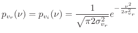 |
(6.45) |
where
 .
.
.
.
.
.
.
.
.
.
.
.
.
.
.
.
.
.
.
.
.
.
.
.
.
.
.
.
.
.
.
.
- ... autocorrelation,7.1
- Note that there are many
possible biased estimates of the true autocorrelation
function. However, we will consider only one of them in this book.
.
.
.
.
.
.
.
.
.
.
.
.
.
.
.
.
.
.
.
.
.
.
.
.
.
.
.
.
.
.
- ... ``complicated''.7.2
- An interesting discussion
of the meaning of randomness is given in Knuth
[131, vol. II].
.
.
.
.
.
.
.
.
.
.
.
.
.
.
.
.
.
.
.
.
.
.
.
.
.
.
.
.
.
.
- ... function.7.3
- In Octave,
it is necessary to install the add-on package octave-forge to
obtain this and other signal processing functions.
.
.
.
.
.
.
.
.
.
.
.
.
.
.
.
.
.
.
.
.
.
.
.
.
.
.
.
.
.
.
- ....7.4
- Note that we
are assuming
 is zero mean. Otherwise, the sample variance would be
defined with the mean subtracted out, as discussed further in
§C.1.10. When the mean is zero, a correlation may be called a
covariance.
is zero mean. Otherwise, the sample variance would be
defined with the mean subtracted out, as discussed further in
§C.1.10. When the mean is zero, a correlation may be called a
covariance.
.
.
.
.
.
.
.
.
.
.
.
.
.
.
.
.
.
.
.
.
.
.
.
.
.
.
.
.
.
.
- ... mean.7.5
- Note that we are not
averaging the PSD to get the total variance, but instead
summing it. This is why the
 factor in the IDFT above
is associated with
factor in the IDFT above
is associated with  and why the IDFT is also written as an
integral with respect to a Hertz frequency axis.
and why the IDFT is also written as an
integral with respect to a Hertz frequency axis.
.
.
.
.
.
.
.
.
.
.
.
.
.
.
.
.
.
.
.
.
.
.
.
.
.
.
.
.
.
.
- ... data.7.6
- A trend is typically estimated using linear
regression. That is, a straight line is fit through the data in a
least squares sense. (See the function polyfit in Matlab or
Octave.)
.
.
.
.
.
.
.
.
.
.
.
.
.
.
.
.
.
.
.
.
.
.
.
.
.
.
.
.
.
.
- ...Kay88:7.7
-
The division by
can be seen as part of the implicit
autocorrelation calculation. It normalizes the peak of the
implicit Bartlett window on the autocorrelation to 1,
as discussed further below. Alternatively, it may be interpreted as a
normalization of the Fourier transform itself, converting a power
spectrum (squared-magnitude FFT) to a normalized power spectrum
(NDFT). Normalization is needed for stationary random processes since they
generally have infinite signal energy but finite average power; i.e.,
 grows without bound as
increases.
grows without bound as
increases.
.
.
.
.
.
.
.
.
.
.
.
.
.
.
.
.
.
.
.
.
.
.
.
.
.
.
.
.
.
.
- ... correlated.7.8
- An exception is when white noise is
filtered using an allpass filter, in which case the output signal is
still white noise.
.
.
.
.
.
.
.
.
.
.
.
.
.
.
.
.
.
.
.
.
.
.
.
.
.
.
.
.
.
.
- ... noise|textbf.7.9
- For a more
formal development, see the Wold decomposition theorem.
.
.
.
.
.
.
.
.
.
.
.
.
.
.
.
.
.
.
.
.
.
.
.
.
.
.
.
.
.
.
- ... noise7.10
- The term ``pink noise'' indicates that the
spectrum is more intense at low frequencies than at high frequencies.
This makes sense since the color pink is heavier in the red end of the
spectrum compared with white which balances all colors equally.
.
.
.
.
.
.
.
.
.
.
.
.
.
.
.
.
.
.
.
.
.
.
.
.
.
.
.
.
.
.
- ...VossAndClarke78,7.11
- Physical phenomena exhibiting a
 power spectral density law include noise in vacuum tubes, carbon resistors,
transistor junctions, metal films, ionic solutions, films at the
superconducting transition, Josephson junctions, nerve membranes,
cosmic background radiation distribution, sunspot activity, and the
flood levels of the river Nile
[294]. In addition, the sub-audio short-time power
fluctuations in music (i.e., below the audible frequencies starting at 20 Hz) have been shown to follow the
characteristic, especially classical music [294].
power spectral density law include noise in vacuum tubes, carbon resistors,
transistor junctions, metal films, ionic solutions, films at the
superconducting transition, Josephson junctions, nerve membranes,
cosmic background radiation distribution, sunspot activity, and the
flood levels of the river Nile
[294]. In addition, the sub-audio short-time power
fluctuations in music (i.e., below the audible frequencies starting at 20 Hz) have been shown to follow the
characteristic, especially classical music [294].
.
.
.
.
.
.
.
.
.
.
.
.
.
.
.
.
.
.
.
.
.
.
.
.
.
.
.
.
.
.
- ... correctly.8.1
- In the Matlab
Signal Processing Toolbox, the argument 'periodic' should be
included when creating the window.
.
.
.
.
.
.
.
.
.
.
.
.
.
.
.
.
.
.
.
.
.
.
.
.
.
.
.
.
.
.
- ...
integer.8.2
- Actually, non-integer
 can be accommodated by
rotating among a set of windows obtained by sampling the underlying
continuous window at different phases.
can be accommodated by
rotating among a set of windows obtained by sampling the underlying
continuous window at different phases.
.
.
.
.
.
.
.
.
.
.
.
.
.
.
.
.
.
.
.
.
.
.
.
.
.
.
.
.
.
.
- ... limited.8.3
- This is of course the Fourier dual
of saying that the uniform sampling of a time-domain signal is
information-preserving provided the signal is properly bandlimited
(in the frequency domain).
.
.
.
.
.
.
.
.
.
.
.
.
.
.
.
.
.
.
.
.
.
.
.
.
.
.
.
.
.
.
- ... magnitude.8.4
- The spectrogram is often called a
sonogram when applied to audio signals.
.
.
.
.
.
.
.
.
.
.
.
.
.
.
.
.
.
.
.
.
.
.
.
.
.
.
.
.
.
.
- ... STFT.8.5
- Perfect reconstruction
is also possible in principle using
 as large as
with the
Hamming window. However, this requires dividing out the amplitude
modulation given by the sum of Hamming windows displaced by
(see
Eq.(7.2)). In practice,
as large as
with the
Hamming window. However, this requires dividing out the amplitude
modulation given by the sum of Hamming windows displaced by
(see
Eq.(7.2)). In practice,  (50% overlap) is the largest hop size
used with the Hamming window because it is the largest value that
preserves the constant-overlap-add (COLA) property. We will
learn in Chapter 9 that
(50% overlap) is the largest hop size
used with the Hamming window because it is the largest value that
preserves the constant-overlap-add (COLA) property. We will
learn in Chapter 9 that  (75% overlap) is significantly
more robust than 50% overlap, and is recommended when spectral
modifications are to be carried out on the STFT data.
(75% overlap) is significantly
more robust than 50% overlap, and is recommended when spectral
modifications are to be carried out on the STFT data.
.
.
.
.
.
.
.
.
.
.
.
.
.
.
.
.
.
.
.
.
.
.
.
.
.
.
.
.
.
.
- ... SPL.8.6
- A listening-level slider would be nice to have in
the Graphical User Interface (GUI) for a loudness spectrogram.
.
.
.
.
.
.
.
.
.
.
.
.
.
.
.
.
.
.
.
.
.
.
.
.
.
.
.
.
.
.
- ...
bank.8.7
- Note that the FFTs are effectively downsampled by this
operation, with the highest ``frequency-domain sampling rate''
occurring at the lowest frequency of the band. Therefore, the FFT
length can be set by matching the adjacent auditory filter spacing to
the low-frequency bin spacing of the FFT at the lower edge of the
frequency range covered by that FFT). In fact, one very large FFT
could be used in which the low-frequency bin spacing is approximately
equal to the spacing of the center-frequencies of the auditory
filter-bank channels at the low-frequency extreme.
.
.
.
.
.
.
.
.
.
.
.
.
.
.
.
.
.
.
.
.
.
.
.
.
.
.
.
.
.
.
- ... level.8.8
- Downloading http://ccrma.stanford.edu/~jos/sasp/hw/SteveJobsHi.wav
and listening at a very low level (approximately 20 dB SPL) verifies that
indeed this sound example sounds like ``Hi...ee-jah,'' in
qualitative agreement with the sone loudness curve in Fig.7.9.
.
.
.
.
.
.
.
.
.
.
.
.
.
.
.
.
.
.
.
.
.
.
.
.
.
.
.
.
.
.
- ... constant.8.9
- Envelope
followers in sound processing classically
behave this way as well [109]. The amplitude envelope is
allowed to increase instantaneously, but it floats down with some time
constant that can be adjusted.
.
.
.
.
.
.
.
.
.
.
.
.
.
.
.
.
.
.
.
.
.
.
.
.
.
.
.
.
.
.
- ...MDFT,9.1
- https://ccrma.stanford.edu/~jos/mdft/Convolution_Theorem.html
.
.
.
.
.
.
.
.
.
.
.
.
.
.
.
.
.
.
.
.
.
.
.
.
.
.
.
.
.
.
- ...).9.2
- These results were obtained using the
fft function in Matlab v5.2 running on a Windows
PC with an 800MHz Athlon CPU.
.
.
.
.
.
.
.
.
.
.
.
.
.
.
.
.
.
.
.
.
.
.
.
.
.
.
.
.
.
.
- ... 2011,9.3
- Octave on a Fedora 15
64-bit Linux machine (built in 2009) with an Intel Core i7-860
quad-core CPU running at 2.8 GHz
.
.
.
.
.
.
.
.
.
.
.
.
.
.
.
.
.
.
.
.
.
.
.
.
.
.
.
.
.
.
- ...MDFT9.4
- https://ccrma.stanford.edu/~jos/mdft/Fast_Fourier_Transform_FFT.html
.
.
.
.
.
.
.
.
.
.
.
.
.
.
.
.
.
.
.
.
.
.
.
.
.
.
.
.
.
.
- ... filter.9.5
- As discussed in [261, Chapter 11],
an FIR filter having impulse response
 is said to be linear
phase when its impulse response is symmetric about some point in time, e.g.,
is said to be linear
phase when its impulse response is symmetric about some point in time, e.g.,
 , for
, for  , where
  is the length of the FIR filter.
.
.
.
.
.
.
.
.
.
.
.
.
.
.
.
.
.
.
.
.
.
.
.
.
.
.
.
.
.
.
- ... (COLA)9.6
- The acronym
COLA is not standard in signal processing, although OLA might be
recognized by many. When writing a paper, acronyms should always be
spelled out on first use, even for surely recognized acronyms such as
``FFT''.
.
.
.
.
.
.
.
.
.
.
.
.
.
.
.
.
.
.
.
.
.
.
.
.
.
.
.
.
.
.
- ... filter|textbf.10.1
- Low-power
applications such as RFID chips use cascaded integrated comb
filters (CIC filters) in their sampling-rate
converters.
.
.
.
.
.
.
.
.
.
.
.
.
.
.
.
.
.
.
.
.
.
.
.
.
.
.
.
.
.
.
- ... filter|textbf.10.2
- In ordinary sampling theory
[270],
each sample of a time-domain signal determines the scaling and
location of a sinc function for all time in the underlying
continuous-time signal represented by the samples. The dc sampling
filter described here is the Fourier dual of the time-domain sinc
function corresponding to a single sample in time.
.
.
.
.
.
.
.
.
.
.
.
.
.
.
.
.
.
.
.
.
.
.
.
.
.
.
.
.
.
.
- ...
demodulation|textbf.10.3
- We use the term ``demodulation'' when frequencies
are translated from high to low (
to 0 in this case).
.
.
.
.
.
.
.
.
.
.
.
.
.
.
.
.
.
.
.
.
.
.
.
.
.
.
.
.
.
.
- ...).10.4
- We
also implicitly assumed that the DFT size
was not smaller than the
window length
.
.
.
.
.
.
.
.
.
.
.
.
.
.
.
.
.
.
.
.
.
.
.
.
.
.
.
.
.
.
.
- ... modifications.10.5
- The term
FBS modifications refers to changing the gain and/or phase
of the time-domain signal coming out of a filter-bank channel. This
is distinct from OLA modifications in which a spectrum is
altered, inverse transformed, and overlap-added into an output buffer.
Multiplicative OLA modifications are exact (no aliasing) when the
zero-padding in the time domain is sufficient. FBS modifications are
not provided zero-padding in the time domain, and for
 there is
aliasing in the channel signals.
there is
aliasing in the channel signals.
.
.
.
.
.
.
.
.
.
.
.
.
.
.
.
.
.
.
.
.
.
.
.
.
.
.
.
.
.
.
- ...
algorithm11.1
- This algorithm was developed by the author circa
1996 for vibrating-string fundamental frequency measurement. It has
been found to work quite well on the middle third (or so) of plucked
string recordings. An extension to stiff strings (stretched
partial overtone frequencies) is described in [266].
.
.
.
.
.
.
.
.
.
.
.
.
.
.
.
.
.
.
.
.
.
.
.
.
.
.
.
.
.
.
- ...MuellerEtAl11,KlapuriMohonk05,KlapuriSAP03,Klapuri01.11.2
- Klapuri's publications home page as of this writing:
http://www.elec.qmul.ac.uk/people/anssik/publications.htm
.
.
.
.
.
.
.
.
.
.
.
.
.
.
.
.
.
.
.
.
.
.
.
.
.
.
.
.
.
.
- ... retrieval|textbf11.3
- For an introduction
to MIR, see, e.g., recent proceedings of the International Conference
on Music Information Retrieval (ISMIR) or Music Information
Retrieval Evaluation eXchange (MIREX) conference.
.
.
.
.
.
.
.
.
.
.
.
.
.
.
.
.
.
.
.
.
.
.
.
.
.
.
.
.
.
.
- ...
construction,11.4
- A matrix is said to be
Toeplitz if the
 ]th
entry can be expressed as a function of
]th
entry can be expressed as a function of  . A Toeplitz matrix is
constant along all diagonals.
. A Toeplitz matrix is
constant along all diagonals.
.
.
.
.
.
.
.
.
.
.
.
.
.
.
.
.
.
.
.
.
.
.
.
.
.
.
.
.
.
.
- ...
recursion.11.5
-
http://ccrma.stanford.edu/~jos/filters/Computing_Reflection_Coefficients.html
.
.
.
.
.
.
.
.
.
.
.
.
.
.
.
.
.
.
.
.
.
.
.
.
.
.
.
.
.
.
- ... hearing:11.6
- Due to nonlinearities in hearing
[179,306], it is not always valid to truncate
the summation at the high-frequency hearing limit. For complete
generally,
should be extended to the highest frequency
present in the signal
 , since inaudible frequencies can give
rise to audible components at the output of a nonlinearity.
, since inaudible frequencies can give
rise to audible components at the output of a nonlinearity.
.
.
.
.
.
.
.
.
.
.
.
.
.
.
.
.
.
.
.
.
.
.
.
.
.
.
.
.
.
.
- ... overtone.11.7
- The
term overtone or partial overtone is generally used to
mean a sinusoidal component which is not harmonically related to the
fundamental frequency.
.
.
.
.
.
.
.
.
.
.
.
.
.
.
.
.
.
.
.
.
.
.
.
.
.
.
.
.
.
.
- ... ways.11.8
- Frequency
modulation is the time-derivative of phase modulation.
.
.
.
.
.
.
.
.
.
.
.
.
.
.
.
.
.
.
.
.
.
.
.
.
.
.
.
.
.
.
- ...McAulayQuatieri86.11.9
- An interesting avenue for future
research is the pursuit of new spectral-modeling primitives and
operators which are generally useful and compact for modeling
important aspects of sound.
.
.
.
.
.
.
.
.
.
.
.
.
.
.
.
.
.
.
.
.
.
.
.
.
.
.
.
.
.
.
- ...SmithSerra.11.10
- Higher-order interpolations of so-called
envelope break-points were also developed at CCRMA in the
late 1970s (e.g., using cubic splines), but for tonal sounds,
linear interpolation is usually sufficient, and the higher-order
envelopes did not see much use, presumably due to the greater
complexity of dealing with them coupled with the lack of significant
benefit.
.
.
.
.
.
.
.
.
.
.
.
.
.
.
.
.
.
.
.
.
.
.
.
.
.
.
.
.
.
.
- ... STFT|textbf,11.11
- Extension to multiresolution FFT analysis was an
important step in obtaining artifact-free analysis and resynthesis
of polyphonic audio sources. Previously, sinusoidal and S+N
modeling had been confined to monophonic sources, such as voice, or
a single instrument, etc.
.
.
.
.
.
.
.
.
.
.
.
.
.
.
.
.
.
.
.
.
.
.
.
.
.
.
.
.
.
.
- ... band11.12
- See
Appendix E for a definition of Bark bands (classical critical bands of
hearing).
.
.
.
.
.
.
.
.
.
.
.
.
.
.
.
.
.
.
.
.
.
.
.
.
.
.
.
.
.
.
- ...Ellis02-pvoc,HejnaAndMusicus9111.13
- Synchronous
Overlap-Add, Fixed Synthesis [104]--a
time-domain method reminiscent of the Eventide ``Harmonizer,''
based on an overlap-add decomposition of the time waveform, with
input windows shifted and output windows regularly spaced for a
fixed output synthesis window-rate. SOLA-FS is said to be more
computationally efficient than SOLA
[240,280].
.
.
.
.
.
.
.
.
.
.
.
.
.
.
.
.
.
.
.
.
.
.
.
.
.
.
.
.
.
.
- ... bank|textbf.11.14
- In Beranek's Acoustics [15, pp. 333-334], the ``one-third octave-band analyzer'' is
defined as the 25-band filter bank having the spectral partition
points (in Hz) [20, 45, 57, 71, 90, 114,
142, 180, 228, 284, 360, 456, 568, 720, 912, 1136, 1440, 1824, 2272,
2880, 3648, 4544, 5760, 7296, 9088, 11520].
.
.
.
.
.
.
.
.
.
.
.
.
.
.
.
.
.
.
.
.
.
.
.
.
.
.
.
.
.
.
- ... bank|textbf,11.15
- An
``octave-band analyzer'' is defined in [15, p. 333] as
the 8-band filter bank having the spectral partition points [37.5,
75, 150, 300, 600, 1200, 2400, 4800, 10000] Hz.
.
.
.
.
.
.
.
.
.
.
.
.
.
.
.
.
.
.
.
.
.
.
.
.
.
.
.
.
.
.
- ... channels.11.16
- Thanks to Jeurgen Herre for
mentioning this reference.
.
.
.
.
.
.
.
.
.
.
.
.
.
.
.
.
.
.
.
.
.
.
.
.
.
.
.
.
.
.
- ...dtftalias):11.17
- A more efficient implementation can use
reshape and sum.
.
.
.
.
.
.
.
.
.
.
.
.
.
.
.
.
.
.
.
.
.
.
.
.
.
.
.
.
.
.
- ... general.11.18
- When the FFT window is
a length N rectangular window, then alias(Hk .* X, Nk) ==
BandK, as defined above, and there is no aliasing after all.
More precisely, the aliased spectral samples all happen to be zeros
of the window transform (which is an aliased sinc function, as
defined in §3.1). These zeros depend on the
window-length being N (no zero-padding), and on the window-type
being rectangular (``no window'').
.
.
.
.
.
.
.
.
.
.
.
.
.
.
.
.
.
.
.
.
.
.
.
.
.
.
.
.
.
.
- ...
bank.11.19
- Do not confuse the Octave program--a free, open-source
implementation of the matlab language--with the musical
octave: a frequency interval spanning a factor of two.
.
.
.
.
.
.
.
.
.
.
.
.
.
.
.
.
.
.
.
.
.
.
.
.
.
.
.
.
.
.
- ... domain.11.20
- The samples are
connected by straight lines to make them visible. The true responses
for the left two bands are aliased sinc functions (asinc). The next
octave up is a sum of two asincs, and the rightmost band (top
octave) is a sum of four asincs. A properly interpolated frequency
response for this filter bank is shown in
Fig.10.33.
.
.
.
.
.
.
.
.
.
.
.
.
.
.
.
.
.
.
.
.
.
.
.
.
.
.
.
.
.
.
- ...dcells11.21
- http://ccrma.stanford.edu/~jos/sasp/dcells.m
.
.
.
.
.
.
.
.
.
.
.
.
.
.
.
.
.
.
.
.
.
.
.
.
.
.
.
.
.
.
- ...dcells2spec11.22
- http://ccrma.stanford.edu/~jos/sasp/dcells2spec.m
.
.
.
.
.
.
.
.
.
.
.
.
.
.
.
.
.
.
.
.
.
.
.
.
.
.
.
.
.
.
- ... wide.11.23
- We do not really have to restrict
consideration to powers of two, as there are many fast Fourier
transform algorithms for various composite and prime lengths
[80,289].
.
.
.
.
.
.
.
.
.
.
.
.
.
.
.
.
.
.
.
.
.
.
.
.
.
.
.
.
.
.
- ... samples''11.24
- Spectral samples are
defined here as ``bin numbers plus 1'', that is, spectral samples
are numbered from 1 as in matlab, rather than from 0, as in the
signal processing literature.
.
.
.
.
.
.
.
.
.
.
.
.
.
.
.
.
.
.
.
.
.
.
.
.
.
.
.
.
.
.
- ...
website.11.25
-
http://ccrma.stanford.edu/~jos/pdf/SMS.pdf
.
.
.
.
.
.
.
.
.
.
.
.
.
.
.
.
.
.
.
.
.
.
.
.
.
.
.
.
.
.
- ....12.1
- We will relax the restriction
 in the next
section. The only reason for the restriction now is to avoid a
different system definition for
in the next
section. The only reason for the restriction now is to avoid a
different system definition for  relative to what we'll derive
in the next section.
relative to what we'll derive
in the next section.
.
.
.
.
.
.
.
.
.
.
.
.
.
.
.
.
.
.
.
.
.
.
.
.
.
.
.
.
.
.
- ....12.2
- The diagram-manipulation derivation in
§11.1.3 would produce
subphase branches,
each scaled by
 , while here we have only
subphase
branches, each feeding a length
, while here we have only
subphase
branches, each feeding a length  FIR filter.
.
.
.
.
.
.
.
.
.
.
.
.
.
.
.
.
.
.
.
.
.
.
.
.
.
.
.
.
.
.
- ...
transients.12.3
- The Dolby AC-3 perceptual audio coding format,
which is formulated more directly as a transform coder (quantized
STFT), switches to a shorter FFT window when transients are detected
in the signal being encoded. The original Dolby AC-2 format used
length 512 FFT windows in a Princen-Bradley time-domain aliasing
cancellation scheme (sampling rate typically 44.1 kHz). The shorter
length for transients in AC-3 was chosen to be 256 samples, or half
the steady-state length [149, §4.1.4]. A special hybrid
window is needed for a smooth transition from steady-state to
transient processing, or vice versa.
.
.
.
.
.
.
.
.
.
.
.
.
.
.
.
.
.
.
.
.
.
.
.
.
.
.
.
.
.
.
- ... level.12.4
- One careful study found that 96-kbps AAC is
roughly equivalent to 128-kbps MP3, which is a 33% lower bitrate at
roughly the same quality level. [149, §4.1.8].
.
.
.
.
.
.
.
.
.
.
.
.
.
.
.
.
.
.
.
.
.
.
.
.
.
.
.
.
.
.
- ... transform|textbf.12.5
- The
 of a
bandpass filter may be defined as its center-frequency divided by its
bandwidth [263].
of a
bandpass filter may be defined as its center-frequency divided by its
bandwidth [263].
.
.
.
.
.
.
.
.
.
.
.
.
.
.
.
.
.
.
.
.
.
.
.
.
.
.
.
.
.
.
- ...
bank|textbf,12.6
- The term ``dyad'' simply means ``two'', as
in monad, dyad, triad, tetrad,
 . Thus, successive bands
in a dyadic filter bank are obtained using a frequency-scale factor of
two.
. Thus, successive bands
in a dyadic filter bank are obtained using a frequency-scale factor of
two.
.
.
.
.
.
.
.
.
.
.
.
.
.
.
.
.
.
.
.
.
.
.
.
.
.
.
.
.
.
.
- ... transforms:B.1
- See
§8.3.1 for the discrete-time case.
.
.
.
.
.
.
.
.
.
.
.
.
.
.
.
.
.
.
.
.
.
.
.
.
.
.
.
.
.
.
- ...MDFT,B.2
- http://ccrma.stanford.edu/~jos/mdft/Cauchy_Schwarz_Inequality.html
.
.
.
.
.
.
.
.
.
.
.
.
.
.
.
.
.
.
.
.
.
.
.
.
.
.
.
.
.
.
- ... filter.B.3
- An allpass filter has unity gain and
arbitrary delay at each frequency.
.
.
.
.
.
.
.
.
.
.
.
.
.
.
.
.
.
.
.
.
.
.
.
.
.
.
.
.
.
.
- ...
Therefore,B.4
- Technically, the Fourier transform of the unit
step function
 does not exist, since
  is not
integrable for any value of
. However, its Laplace
transform
is not
integrable for any value of
. However, its Laplace
transform
 does exist in the right-half
  plane, and
the limit as
plane, and
the limit as
 is well behaved and can be taken as the
definition of the Fourier transform. The same construction works for
is well behaved and can be taken as the
definition of the Fourier transform. The same construction works for
 ,
,
 , and so on.
.
.
.
.
.
.
.
.
.
.
.
.
.
.
.
.
.
.
.
.
.
.
.
.
.
.
.
.
.
.
- ... orderB.5
- We will say that a function
 is of order
 if
there exists
if
there exists  and some positive constant
  such
that
such
that
 for all
 .
.
.
.
.
.
.
.
.
.
.
.
.
.
.
.
.
.
.
.
.
.
.
.
.
.
.
.
.
.
.
.
- ....B.6
- Such a decomposition may be
constructed by differentiating to obtain
 and defining
![$\displaystyle w^\prime_{\scriptscriptstyle\uparrow}(t)\isdef \left\{\begin{array}{ll} w^\prime , & w^\prime \geq 0 \\ [5pt] 0, & w^\prime <0 \\ \end{array} \right.$](img2589.png) |
(B.81) |
and similarly for
 . (The derivatives may include impulses
corresponding to discontinuities in
. (The derivatives may include impulses
corresponding to discontinuities in  .)
.)
The quantity
![$ [w_{\scriptscriptstyle\uparrow}(b)-w_{\scriptscriptstyle\uparrow}(a)] + [w_{\scriptscriptstyle\downarrow}(b)-w_{\scriptscriptstyle\downarrow}(a)]$](img2591.png) is called the
total variation of
is called the
total variation of  on
on  ; if this value is finite,
then
is said to be of
bounded variation on
.
; if this value is finite,
then
is said to be of
bounded variation on
.
.
.
.
.
.
.
.
.
.
.
.
.
.
.
.
.
.
.
.
.
.
.
.
.
.
.
.
.
.
.
- ...impulse.C.1
- The impulse
 may be defined as any ``function''
  for which
 |
(C.10) |
where  is assumed continuous at
  . A typical definition is
![$\displaystyle \delta(x) \isdef \lim_{\Delta \to 0} \left\{\begin{array}{ll} \frac{1}{\Delta}, & 0\leq x\leq \Delta \\ [5pt] 0, & \hbox{otherwise}. \\ \end{array} \right.$](img2629.png) |
(C.11) |
The impulse was introduced in Chapter 2 starting at §B.10.
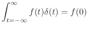
See also [264,36,150] for further development.
.
.
.
.
.
.
.
.
.
.
.
.
.
.
.
.
.
.
.
.
.
.
.
.
.
.
.
.
.
.
- ... process.C.2
- The general class of stochastic processes for
which time averages equal ensemble averages is called ergodic
stochastic processes [201]. In this book, all
stochastic processes are assumed ergodic (and hence stationary)
because they can all be modeled as filtered white noise, where the
filter is stable, linear, and (at least approximately over short
durations) time-invariant. Furthermore, the driving noise can be
chosen to be Gaussian; see more advanced texts on stochastic
processes regarding distinctions that can arise in non-ergodic
cases.
.
.
.
.
.
.
.
.
.
.
.
.
.
.
.
.
.
.
.
.
.
.
.
.
.
.
.
.
.
.
- ... length.C.3
- Note
that 20 ms contains only one period of a sinusoid at 50 Hz, which is
above lower limit of pitch perception (the low note of the piano, A0,
is tuned to 22 Hz). It is therefore possible to encounter difficulty
resolving tones in the deep bass region of the audio spectrum. A 20
ms frame length works quite well, however, for telephone speech
processing, in which the nominal bandwidth is 200-3200 Hz; in this
case, a 20ms frame has at least four periods of the lowest frequency
present, and harmonic resolution is assured under the Hamming window.
In wideband audio work, a multiresolution analysis is often highly
preferable.
.
.
.
.
.
.
.
.
.
.
.
.
.
.
.
.
.
.
.
.
.
.
.
.
.
.
.
.
.
.
- ... numbers.C.4
-
Two random events
 and
and  are said to be
independent if the
probability of event
and
occurring together equals the product
of the probability of event
times the probability of event
.
Similarly, two random variables
are said to be
independent if the
probability of event
and
occurring together equals the product
of the probability of event
times the probability of event
.
Similarly, two random variables  and
and  are said to be
independent if the
probability that both
are said to be
independent if the
probability that both  and
and  equals the probability that
times the probability that
, where
equals the probability that
times the probability that
, where  and
and  are any
values that the respective random variables can assume. For purposes
of this book, it is sufficient to have only an intuitive
understanding of terms such as these from probability theory. Only
sample correlations will be needed for noise spectrum analysis.
are any
values that the respective random variables can assume. For purposes
of this book, it is sufficient to have only an intuitive
understanding of terms such as these from probability theory. Only
sample correlations will be needed for noise spectrum analysis.
.
.
.
.
.
.
.
.
.
.
.
.
.
.
.
.
.
.
.
.
.
.
.
.
.
.
.
.
.
.
- ...diffthm).D.1
- This approach to the proof was discovered on the Web,
for the real case, at
http://www.ph.tn.tudelft.nl/~lucas/education/tn254/2002/Fourier%20transform%20of%20a%20Gaussian.pdf
.
.
.
.
.
.
.
.
.
.
.
.
.
.
.
.
.
.
.
.
.
.
.
.
.
.
.
.
.
.
- ... theoremD.2
- http://mathworld.wolfram.com/CentralLimitTheorem.html
.
.
.
.
.
.
.
.
.
.
.
.
.
.
.
.
.
.
.
.
.
.
.
.
.
.
.
.
.
.
- ...
increases.D.3
- This can be shown as a consequence of the central
limit theorem. Coincidentally, the Gaussian function is believed to
have first appeared for approximating large binomial coefficients in
the 2nd edition (1718) of Doctrine of Chances
by Abraham de Moivre (a book on probability).
.
.
.
.
.
.
.
.
.
.
.
.
.
.
.
.
.
.
.
.
.
.
.
.
.
.
.
.
.
.
- ...,D.4
- http://mathworld.wolfram.com/NormalDistribution.html
.
.
.
.
.
.
.
.
.
.
.
.
.
.
.
.
.
.
.
.
.
.
.
.
.
.
.
.
.
.
- ... BarksE.1
- The
normalized warped-frequency interval
![$ \omega\in[0,\pi]$](img2920.png) was converted to
Barks
by the affine transformation
was converted to
Barks
by the affine transformation
 ,
where
,
where  is the number of Bark bands in use. For example,
  for
a
for
a  kHz sampling rate.
.
.
.
.
.
.
.
.
.
.
.
.
.
.
.
.
.
.
.
.
.
.
.
.
.
.
.
.
.
.
- ...JOST:E.2
- Matlab functions bark2lin.m and lin2bark.m for transforming between linear and bark-warped frequency
representations are available on the internet at http://ccrma.stanford.edu/~jos/bbt/bbt.html.
.
.
.
.
.
.
.
.
.
.
.
.
.
.
.
.
.
.
.
.
.
.
.
.
.
.
.
.
.
.
- ...Darrigol07.G.1
- For an
online biography of Daniel Bernoulli, see also
http://www-groups.dcs.st-and.ac.uk/~history/Biographies/Bernoulli_Daniel.html
.
.
.
.
.
.
.
.
.
.
.
.
.
.
.
.
.
.
.
.
.
.
.
.
.
.
.
.
.
.
- ...G.2
- This was before Fourier theory (1822), and before
differential equations as we now know them. Calculus using
trigonometric functions was still a new topic at the time.
D'Alembert derived his results from Newton's second law applied to a
differential string element, integrating the result, and imposing
rigid boundary constraints.
.
.
.
.
.
.
.
.
.
.
.
.
.
.
.
.
.
.
.
.
.
.
.
.
.
.
.
.
.
.
- ...
loudspeakers).G.3
- Of course, we know now that the sound of a
vibrating string is produced mainly by the bridge excitation, which
is driven by a superposition of the vibrating string modes, as
envisioned by Bernoulli, or, in an equally valid alternative
formulation, by the traveling waves of D'Alembert.
.
.
.
.
.
.
.
.
.
.
.
.
.
.
.
.
.
.
.
.
.
.
.
.
.
.
.
.
.
.
- ... masks.G.4
- See also the
fascinating history of ``optical synthesis'' at
http://www.umatic.nl/tonewheels_historical.html,
including the photos of Arseny Avraamov's hand-drawn motion picture
soundtracks (1930) and Oskar Fischinger's ``sound scrolls'' (1932).
Also, the Theremin Center has photos of Boris Yankovsky's
``vibroexponator'' soundtracks using syntones and spectral mutations
(http://www.theremin.ru/archive/vibroexponator.htm).
.
.
.
.
.
.
.
.
.
.
.
.
.
.
.
.
.
.
.
.
.
.
.
.
.
.
.
.
.
.
- ... Hz)G.5
- According to the voder patent (US Patent
2,121,142), the ten bandpass edges were, in Hz,
0, 225, 450, 700, 1000, 1400, 2000, 2700, 3800, 5400, and 7500.
The voder patent refers to a vocoder patent application, serial number
47,393, filed October 30, 1935, but it appears that the vocoder patent
may have never issued. In any case, Figure 1 of the voder patent is
described as ``similar'' to that of the vocoder, and having ``been
used as the natural development from the analyzer-synthesizer circuit
referred to in my previous application, Serial No. 47,393'' and the
improved version (Figure 6 of the voder patent) specified the same ten
bandlimits.
.
.
.
.
.
.
.
.
.
.
.
.
.
.
.
.
.
.
.
.
.
.
.
.
.
.
.
.
.
.
- ... technicians.G.6
- For a
photo, see
http://davidszondy.com/future/robot/voder.htm.
See also the Smithsonian Speech Synthesis History Project:
https://amhistory.si.edu/archives/speechsynthesis/ss_home.htm
.
.
.
.
.
.
.
.
.
.
.
.
.
.
.
.
.
.
.
.
.
.
.
.
.
.
.
.
.
.
- ... domain.G.7
- Dolson and Laroche have extended
this idea to the processing of nonparametric spectral peaks in
the short-time spectrum
[143,142,139].
.
.
.
.
.
.
.
.
.
.
.
.
.
.
.
.
.
.
.
.
.
.
.
.
.
.
.
.
.
.
- ...G.8
- In practice, one normally cross-fades among tables
designed for different pitch ranges, as described, e.g., at
http://swiki.hfbk-hamburg.de/MusicTechnology/878
.
.
.
.
.
.
.
.
.
.
.
.
.
.
.
.
.
.
.
.
.
.
.
.
.
.
.
.
.
.
- ...G.9
- In practical additive synthesis, each harmonic overtone, or
harmonic overtone group, may be synthesized using a wavetable
oscillator
(§G.8.4) [165,27,193].
When the number of overtones is large, the inverse-FFT method is
typically used [239].
.
.
.
.
.
.
.
.
.
.
.
.
.
.
.
.
.
.
.
.
.
.
.
.
.
.
.
.
.
.
- ...
signals.G.10
- An early SAIL program reduce.sai for
adaptively allocating piecewise-linear breakpoints is available
online at
http://ccrma.stanford.edu/~jos/sasp/reduce.sai
.
.
.
.
.
.
.
.
.
.
.
.
.
.
.
.
.
.
.
.
.
.
.
.
.
.
.
.
.
.
- ...
convolution).G.11
- A model typically means parametric
model. In contrast, a nonparametric representation, such
as an FFT, is regarded as data or processed data--not
a model. The number of data points (``degrees of freedom'') in a
nonparametric model is typically on the same order as that of the
original data. True model parameters, on the other hand,
will have far fewer degrees of freedom than the original data.
.
.
.
.
.
.
.
.
.
.
.
.
.
.
.
.
.
.
.
.
.
.
.
.
.
.
.
.
.
.
- ...
1977,G.12
- This is a personal observation based on using the
software written by James A. Moorer running on the PDP KL-10 soon
after I arrived at CCRMA. (At that time, ``CCRMA'' was an unnamed
computer-music project at the Stanford Artificial Intelligence
Lab). From reading the code, it appeared to be an implementation along
the lines of Portnoff's 1976 paper. As far as I know, prior
additive-synthesis analysis was performed by
the heterodyne-comb technique [185], which is related
to Goetzel's algorithm for computing a single bin of the DFT
recursively.
.
.
.
.
.
.
.
.
.
.
.
.
.
.
.
.
.
.
.
.
.
.
.
.
.
.
.
.
.
.
- ... transient.G.13
- The noise component
cannot be used, in general, because no matter how much resolution is
provided in the amplitude envelope of the noise, there is usually no
guarantee that the noise, being random, will have the desired
amplitude at the critical time it is needed.
.
.
.
.
.
.
.
.
.
.
.
.
.
.
.
.
.
.
.
.
.
.
.
.
.
.
.
.
.
.
- ...PARSHLH.1
- PARSHL was so named because it could follow
partials (as opposed to merely harmonics). Being written for
the PDP-10 computer running the SAIL operating system, the filename
was restricted to 6 characters, so that ``partial'' became
``PARSHL''.
.
.
.
.
.
.
.
.
.
.
.
.
.
.
.
.
.
.
.
.
.
.
.
.
.
.
.
.
.
.
- ... phaseH.2
- The
version written in 1985 did not support phase. Phase support was
added much later by the second author of [271] in the
context of his Ph.D. research, using the phase interpolation algorithm
of McAulay and Quatieri [174].
.
.
.
.
.
.
.
.
.
.
.
.
.
.
.
.
.
.
.
.
.
.
.
.
.
.
.
.
.
.
- ...
forever,H.3
- We tried reusing turned-off oscillators but found
them to be more trouble than they were worth in our environment.
.
.
.
.
.
.
.
.
.
.
.
.
.
.
.
.
.
.
.
.
.
.
.
.
.
.
.
.
.
.