Next |
Prev |
Up |
Top
|
Index |
JOS Index |
JOS Pubs |
JOS Home |
Search
Relation of Smoothness to Roll-Off Rate
In §3.1.1, we found that the side lobes of
the rectangular-window transform ``roll off'' as  . In this
section we show that this roll-off rate is due to the amplitude
discontinuity at the edges of the window. We also show that, more
generally, a discontinuity in the
. In this
section we show that this roll-off rate is due to the amplitude
discontinuity at the edges of the window. We also show that, more
generally, a discontinuity in the  th derivative corresponds to a
roll-off rate of
th derivative corresponds to a
roll-off rate of
 .
.
The Fourier transform of an impulse
 is simply
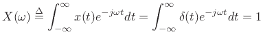 |
(B.70) |
by the sifting property of the impulse under integration. This shows
that an impulse consists of Fourier components at all frequencies in
equal amounts. The roll-off rate is therefore zero in the
Fourier transform of an impulse.
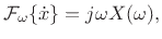
By the differentiation theorem for Fourier transforms
(§B.2), if
 , then
 |
(B.71) |
where
 . Consequently, the integral
of
. Consequently, the integral
of  transforms to
 :
:
 |
(B.72) |
The integral of the impulse is the unit step function:
![$\displaystyle \int_{-\infty}^t \delta(\tau)\,d\tau = u(t) \isdef \left\{\begin{array}{ll} 1, & t\geq0 \\ [5pt] 0, & t<0 \\ \end{array} \right.$](img2569.png) |
(B.73) |
Therefore,B.4
 |
(B.74) |
Thus, the unit step function has a roll-off rate of  dB per
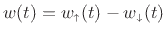
octave, just like the rectangular window. In fact, the rectangular
window can be synthesized as the superposition of two step functions:
dB per
octave, just like the rectangular window. In fact, the rectangular
window can be synthesized as the superposition of two step functions:
 |
(B.75) |
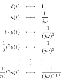
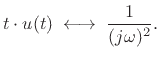
Integrating the unit step function gives a linear ramp function:
![$\displaystyle \int_{-\infty}^t u(\tau)d\tau = t \cdot u(t) = \left\{\begin{array}{ll} t, & t\geq0 \\ [5pt] 0, & t<0 \\ \end{array} \right..$](img2577.png) |
(B.76) |
Applying the integration theorem again yields
 |
(B.77) |
Thus, the linear ramp has a roll-off rate of  dB per octave.
Continuing in this way, we obtain the following Fourier pairs:
dB per octave.
Continuing in this way, we obtain the following Fourier pairs:
Now consider the Taylor series expansion of the function
 at
at
 :
:
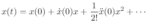 |
(B.78) |
The derivatives up to order  are all zero at
. The
th
derivative, however, has a discontinuous jump at
. Since this is
the only ``wideband event'' in the signal, we may conclude that a
discontinuity in the
th derivative corresponds to a roll-off rate
of
. The following theorem generalizes this result to
a wider class of functions which, for our purposes, will be spectrum
analysis window functions (before sampling):
are all zero at
. The
th
derivative, however, has a discontinuous jump at
. Since this is
the only ``wideband event'' in the signal, we may conclude that a
discontinuity in the
th derivative corresponds to a roll-off rate
of
. The following theorem generalizes this result to
a wider class of functions which, for our purposes, will be spectrum
analysis window functions (before sampling):
Theorem: (Riemann Lemma):
If the derivatives up to order
of the function  exist and
are of bounded variation (defined below), then its Fourier Transform
exist and
are of bounded variation (defined below), then its Fourier Transform
 is asymptotically of orderB.5
, i.e.,
is asymptotically of orderB.5
, i.e.,
 |
(B.79) |
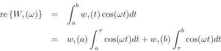
Proof: Following
[202, p. 95], let
be any real function of bounded
variation on the interval  of the real line, and let
 |
(B.80) |
denote its decomposition into a nondecreasing part
 and
nonincreasing part
and
nonincreasing part
 .B.6 Then there exists
 such that
Since
 |
(B.82) |
we conclude
 |
(B.83) |
where
 , which is finite since
 is of bounded variation. Note that the conclusion holds also
when
is of bounded variation. Note that the conclusion holds also
when
 . Analogous conclusions follow for
im
. Analogous conclusions follow for
im ,
re
,
re , and
im
, leading to the result
, and
im
, leading to the result
 |
(B.84) |
If in addition the derivative
 is bounded on
, then
the above gives that its transform
is bounded on
, then
the above gives that its transform
 is
asymptotically of order
, so that
is
asymptotically of order
, so that
 . Repeating this argument, if the first
derivatives exist and are of bounded variation on
, we have
. Repeating this argument, if the first
derivatives exist and are of bounded variation on
, we have
 .
.

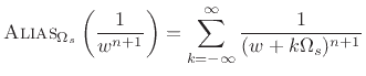
Since spectrum-analysis windows  are often obtained by
sampling continuous time-limited functions
, we
normally see these asymptotic roll-off rates in aliased
form, e.g.,
are often obtained by
sampling continuous time-limited functions
, we
normally see these asymptotic roll-off rates in aliased
form, e.g.,
 |
(B.85) |
where
 denotes the sampling rate in radians per
second. This aliasing normally causes the roll-off rate to ``slow
down'' near half the sampling rate, as shown in
Fig.3.6
for the rectangular window transform. Every window transform must be
continuous at
denotes the sampling rate in radians per
second. This aliasing normally causes the roll-off rate to ``slow
down'' near half the sampling rate, as shown in
Fig.3.6
for the rectangular window transform. Every window transform must be
continuous at
 (for finite windows), so the roll-off
envelope must reach a slope of zero there.
(for finite windows), so the roll-off
envelope must reach a slope of zero there.
In summary, we have the following Fourier rule-of-thumb:
 |
(B.86) |
This is also  dB per decade.
To apply this result to estimating FFT window roll-off rate
(as in Chapter 3), we normally only need to look at the window's
endpoints. The interior of the window is usually
differentiable of all orders. For discrete-time windows, the roll-off
rate ``slows down'' at high frequencies due to aliasing.
Next |
Prev |
Up |
Top
|
Index |
JOS Index |
JOS Pubs |
JOS Home |
Search
[How to cite this work] [Order a printed hardcopy] [Comment on this page via email]