 |
(4.2) |
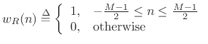
The (zero-centered) rectangular window may be defined by
|
(4.2) |
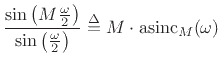
To see what happens in the frequency domain, we need to look at the DTFT of the window:

where the last line was derived using the closed form of a geometric series:
 |
(4.3) |
| (4.6) |
The term ``aliased sinc function'' refers to the fact that it may be
simply obtained by sampling the length-![]() continuous-time rectangular window, which has Fourier transform
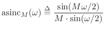
sinc
continuous-time rectangular window, which has Fourier transform
sinc![]() (given amplitude
(given amplitude
![]() in the time domain). Sampling at intervals of
in the time domain). Sampling at intervals of ![]() seconds in
the time domain corresponds to aliasing in the frequency domain over
the interval
seconds in
the time domain corresponds to aliasing in the frequency domain over
the interval ![]() Hz, and by direct derivation, we have found the
result. It is interesting to consider what happens as the window
duration increases continuously in the time domain: the magnitude
spectrum can only change in discrete jumps as new samples are
included, even though it is continuously parametrized in
Hz, and by direct derivation, we have found the
result. It is interesting to consider what happens as the window
duration increases continuously in the time domain: the magnitude
spectrum can only change in discrete jumps as new samples are
included, even though it is continuously parametrized in ![]() .
.
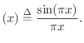
As the sampling rate goes to infinity, the aliased sinc function therefore approaches the sinc function
Figure 3.2 illustrates
![]() for
for ![]() . Note that this is the complete
window transform, not just its real part. We obtain real window
transforms like this only for zero-centered, symmetric windows. Note
that the phase of rectangular-window transform
. Note that this is the complete
window transform, not just its real part. We obtain real window
transforms like this only for zero-centered, symmetric windows. Note
that the phase of rectangular-window transform
![]() is
zero for
is
zero for
![]() , which is the width of the
main lobe. This is why zero-centered windows are often called
zero-phase windows; while the phase
actually alternates between 0
and
, which is the width of the
main lobe. This is why zero-centered windows are often called
zero-phase windows; while the phase
actually alternates between 0
and ![]() radians, the
radians, the ![]() values
occur only within side-lobes which are routinely neglected (in fact,
the window is normally designed to ensure that all side-lobes can be
neglected).
values
occur only within side-lobes which are routinely neglected (in fact,
the window is normally designed to ensure that all side-lobes can be
neglected).
More generally, we may plot both the magnitude and phase of the window versus frequency, as shown in Figures 3.4 and 3.5 below. In audio work, we more typically plot the window transform magnitude on a decibel (dB) scale, as shown in Fig.3.3 below. It is common to normalize the peak of the dB magnitude to 0 dB, as we have done here.
![\includegraphics[width=3.5in]{eps/rectWindow}](img304.png)
![$\displaystyle \frac{e^{-j \omega \frac{1}{2}}}{e^{-j\omega \frac{1}{2}}}
\left[ \frac{ e^{j \omega \frac{M}{2}}-e^{-j\omega\frac{M}{2}}}
{e^{j \omega\frac{1}{2}}-e^{-j\omega\frac{1}{2}}} \right]$](img309.png)
 sinc
sinc![\includegraphics[width=\textwidth ,height=2.25in]{eps/rectWindowRawFT}](img327.png)
![\includegraphics[width=\twidth]{eps/rectWindowFT}](img332.png)
![% latex2html id marker 72776
\includegraphics[width=\twidth,height=0.3125\theight]{eps/rectWindowFTzeroX}](img333.png)
![% latex2html id marker 72780
\includegraphics[width=\twidth,height=0.3125\theight]{eps/rectWindowPhaseFT}](img334.png)