![\begin{psfrags}
% latex2html id marker 17202\psfrag{a} []{ \Large$ \alpha $}\psfrag{b} []{ \Large$ \beta $}\psfrag{g} []{ \Large$ \gamma $\ }\begin{figure}[htbp]
\includegraphics[width=\textwidth ]{eps/parabola}
\caption{Illustration of
parabolic peak interpolation using the three samples nearest the peak.}
\end{figure}
\end{psfrags}](img1002.png)
In quadratic interpolation of sinusoidal spectrum-analysis peaks, we replace the main lobe of our window transform by a quadratic polynomial, or ``parabola''. This is valid for any practical window transform in a sufficiently small neighborhood about the peak, because the higher order terms in a Taylor series expansion about the peak converge to zero as the peak is approached.
Note that, as mentioned in §D.1, the Gaussian window transform magnitude is precisely a parabola on a dB scale. As a result, quadratic spectral peak interpolation is exact under the Gaussian window. Of course, we must somehow remove the infinitely long tails of the Gaussian window in practice, but this does not cause much deviation from a parabola, as shown in Fig.3.36.
Referring to Fig.5.15, the general formula for a parabola may be written as
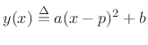 |
(6.29) |
At the three samples nearest the peak, we have
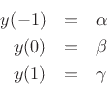
where we arbitrarily renumbered the bins about the peak ![]() , 0, and 1.
Writing the three samples in terms of the interpolating parabola gives
, 0, and 1.
Writing the three samples in terms of the interpolating parabola gives
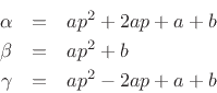
which implies
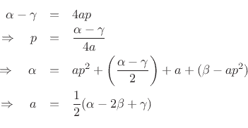
Hence, the interpolated peak location is given in bins6.9 (spectral samples) by
![$\displaystyle \zbox {p=\frac{1}{2}\frac{\alpha-\gamma}{\alpha-2\beta+\gamma}} \in [-1/2,1/2].$](img1010.png) |
(6.30) |
Using the interpolated peak location, the peak magnitude estimate is
 |
(6.31) |