- ... direction.2.1
- To determine whether a surface is
effectively flat, it may first be smoothed so that variations less
than a wavelength in size are ignored. That is, waves do not ``see''
variations on a scale much less than a wavelength.
.
.
.
.
.
.
.
.
.
.
.
.
.
.
.
.
.
.
.
.
.
.
.
.
.
.
.
.
.
.
- ...2.2
- In the code of Fig. 1.9, the first executable line
changes the global STK sampling-rate from 44100 Hz (the default) to
that of the input soundfile. If this is not done, there is a hidden
sampling-rate conversion using linear interpolation when the input
file is read, if its sampling rate is different from the global STK
sampling-rate. This default rate conversion could alternatively be
canceled by saying input.setRate(1.0); after the input file
is opened.
.
.
.
.
.
.
.
.
.
.
.
.
.
.
.
.
.
.
.
.
.
.
.
.
.
.
.
.
.
.
- ....2.3
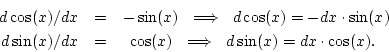
- It is easy to see that the exponential function
 has the property
 . To show that all
differentiable functions with this property are exponentials, one can
look at the definition of the derivative of
. To show that all
differentiable functions with this property are exponentials, one can
look at the definition of the derivative of  with respect to
 :
Since
:
Since
 , we must have
  . Therefore, the last
limit above converges to some constant
. Therefore, the last
limit above converges to some constant
 , and
, and
 . In this way, it is shown that
  satisfies a differential equation whose solution space consists of
exponential functions of the form
satisfies a differential equation whose solution space consists of
exponential functions of the form
 , and to obtain
, we must have
, and to obtain
, we must have  .
.
.
.
.
.
.
.
.
.
.
.
.
.
.
.
.
.
.
.
.
.
.
.
.
.
.
.
.
.
.
.
- ... dispersion2.4
- Dispersion
occurs in a traveling wave whenever the propagation speed is different
at two or more frequencies.
.
.
.
.
.
.
.
.
.
.
.
.
.
.
.
.
.
.
.
.
.
.
.
.
.
.
.
.
.
.
- ... as2.5
- Note that
Fig. 1.18 is given in direct form 2, so its describing equations are
 . To make the figure
correspond exactly to the direct-form-1 difference equation, simply
move
. To make the figure
correspond exactly to the direct-form-1 difference equation, simply
move  from the output arrow to the input arrow. That is, commute
the scaling by and the feedback loop so that is first.
from the output arrow to the input arrow. That is, commute
the scaling by and the feedback loop so that is first.
.
.
.
.
.
.
.
.
.
.
.
.
.
.
.
.
.
.
.
.
.
.
.
.
.
.
.
.
.
.
- ... filter|textbf,2.6
- Readers of this book are not expected to know linear algebra,
but one does not have to learn much to follow the discussion in this
section. See, for example, [422, available online] for the
basic matrix operations. An excellent linear algebra text is
[308].
.
.
.
.
.
.
.
.
.
.
.
.
.
.
.
.
.
.
.
.
.
.
.
.
.
.
.
.
.
.
- ....2.7
- The
 superscript denotes matrix
transposition (see any linear algebra text).
superscript denotes matrix
transposition (see any linear algebra text).
.
.
.
.
.
.
.
.
.
.
.
.
.
.
.
.
.
.
.
.
.
.
.
.
.
.
.
.
.
.
- ... line.2.8
- This
structure may be quickly derived by forming a series combination of a
feedback comb filter followed by a feedforward comb filter, and
noticing that the two delay lines contain the same numbers at all
times. Therefore, the two delay lines can be replaced by a single
shared delay line.
.
.
.
.
.
.
.
.
.
.
.
.
.
.
.
.
.
.
.
.
.
.
.
.
.
.
.
.
.
.
- ...causal|textbf2.9
- A filter is said
to be causal if its impulse response
 is zero for
  .
.
.
.
.
.
.
.
.
.
.
.
.
.
.
.
.
.
.
.
.
.
.
.
.
.
.
.
.
.
.
.
- ...fbffcf.2.10
- Gerzon's starting point was Schroeder's
allpass which differs slightly from Eq. (1.13), having difference
equation [386]
with  required for stability. This structure can be derived
from Eq. (1.13) on page
required for stability. This structure can be derived
from Eq. (1.13) on page ![[*]](../icons/crossref.png) by moving the feedforward path to
the other side of the input summer and deriving the new gain for
by moving the feedforward path to
the other side of the input summer and deriving the new gain for
 . Gerzon's idea was to replace the
  -sample delay by a
multi-input, multi-output (MIMO) allpass-filter matrix;
Gerzon's ``unitary frequency-response matrices'' correspond to
paraunitary matrix transfer functions
[426, Appendix D].
-sample delay by a
multi-input, multi-output (MIMO) allpass-filter matrix;
Gerzon's ``unitary frequency-response matrices'' correspond to
paraunitary matrix transfer functions
[426, Appendix D].
.
.
.
.
.
.
.
.
.
.
.
.
.
.
.
.
.
.
.
.
.
.
.
.
.
.
.
.
.
.
- ... response|textbf2.11
- A (possibly complex) matrix
 is said
to be unitary if
is said
to be unitary if
 , where the `
 '
superscript denotes complex-conjugate transposition:
'
superscript denotes complex-conjugate transposition:
 (also called the Hermitian transpose). A real
unitary matrix is said to be orthogonal, and this is the case
most commonly used in practice.
(also called the Hermitian transpose). A real
unitary matrix is said to be orthogonal, and this is the case
most commonly used in practice.
.
.
.
.
.
.
.
.
.
.
.
.
.
.
.
.
.
.
.
.
.
.
.
.
.
.
.
.
.
.
- ... impedance2.12
-
See §J.1 for definitions and discussion regarding
impedance.
.
.
.
.
.
.
.
.
.
.
.
.
.
.
.
.
.
.
.
.
.
.
.
.
.
.
.
.
.
.
- ... ear,3.1
- It is also possible to use one delay
line for a single source to multiple ears, or multiple sources to one
ear.
.
.
.
.
.
.
.
.
.
.
.
.
.
.
.
.
.
.
.
.
.
.
.
.
.
.
.
.
.
.
- ... time3.2
- Reverberation time is typically defined as
 , the time, in seconds, to decay by 60 dB.
.
.
.
.
.
.
.
.
.
.
.
.
.
.
.
.
.
.
.
.
.
.
.
.
.
.
.
.
.
.
- ... shown3.3
- A simple proof for rectangular rooms can be based on
considering a single spherical wave produced from a point source in
the room. Imagine tesselating all of 3D space with copies of the
original room (minus the source), all in the same orientation. As the
spherical wave expands, it intersects a number of rooms that is
roughly proportional to its radius squared. Since the radius is
proportional to time for an expanding spherical wavefront (
 ),
the number of rooms containing a wave section grows as
),
the number of rooms containing a wave section grows as  . By
adding all the rooms together (flipping every other one along and
. By
adding all the rooms together (flipping every other one along and
 ), we obtain the acoustic field in the original reverberant room at
time
), we obtain the acoustic field in the original reverberant room at
time  , for the case of lossless wall reflections of pressure waves.
(This is the dual of the usual image method for computing the
impulse response of a room [14].) Since each
wave-section traverses each point exactly once in each room image
(disregarding reflections, which are accounted for by different room
images), the number of echoes at any point in the room during the time
it takes a plane wave to traverse the room is very close to the number
of wave sections in the room at the beginning of that time interval.
, for the case of lossless wall reflections of pressure waves.
(This is the dual of the usual image method for computing the
impulse response of a room [14].) Since each
wave-section traverses each point exactly once in each room image
(disregarding reflections, which are accounted for by different room
images), the number of echoes at any point in the room during the time
it takes a plane wave to traverse the room is very close to the number
of wave sections in the room at the beginning of that time interval.
.
.
.
.
.
.
.
.
.
.
.
.
.
.
.
.
.
.
.
.
.
.
.
.
.
.
.
.
.
.
- ... shown3.4
- As described in virtually any acoustics textbook, the resonant modes of a
rectangular room are given by (see, e.g., [327, pp. 284-286])
 |
(3.1) |
where
 denotes the
  th harmonic frequency (radian/meter)
of the fundamental standing wave in the direction (
th harmonic frequency (radian/meter)
of the fundamental standing wave in the direction ( being the
length of the room along ), and similarly for the and
being the
length of the room along ), and similarly for the and  directions. Thus, the mode frequencies of a room can be enumerated on
a uniform 3D Cartesian grid indexed by
directions. Thus, the mode frequencies of a room can be enumerated on
a uniform 3D Cartesian grid indexed by  . The grid spacings
along , , and are taken to be
. The grid spacings
along , , and are taken to be  ,
,  , and
, and
 , respectively. From Eq. (2.1), the spatial frequency
 of mode is given by the distance from the origin
of the grid to the point indexed by . Therefore, the number of room
modes having spatial frequency between and
of mode is given by the distance from the origin
of the grid to the point indexed by . Therefore, the number of room
modes having spatial frequency between and  is equal to
the number of grid points lying in the spherical annulus between
radius and . Since the grid is uniform, this number
grows as
is equal to
the number of grid points lying in the spherical annulus between
radius and . Since the grid is uniform, this number
grows as  .
.
.
.
.
.
.
.
.
.
.
.
.
.
.
.
.
.
.
.
.
.
.
.
.
.
.
.
.
.
.
.
- ...3.5
- One definition of when late
reverberation begins is when it begins to look Gaussian, since
a random sum of plane waves uniformly distributed over all angles of
arrival yields a Gaussian distributed pressure field. (The fact that
late reverberation in a rectangular room always approaches a
superposition of plane waves traveling in all directions can be seen
from the ``image-method dual'' argument in §2.2.1.) One way to
test for Gaussianness is to form a histogram of impulse
response sample values over a finite window (say 10ms, or roughly 500
samples), and compare the normalized histogram
 to a standard
Gaussian bell curve
to a standard
Gaussian bell curve  computed using the measured sample
variance. A threshold can be placed on
computed using the measured sample
variance. A threshold can be placed on
 , or some
number of higher order sample moments can be compared. A simpler test
is to determine when roughly 30% of the samples in a frame have
magnitude larger than one standard deviation (
, or some
number of higher order sample moments can be compared. A simpler test
is to determine when roughly 30% of the samples in a frame have
magnitude larger than one standard deviation (
 )
[2],
since the probability of this occurring in truly Gaussian sequences is
)
[2],
since the probability of this occurring in truly Gaussian sequences is
 erf
erf , where
erf
, where
erf denotes the ``error function'' (integral from
  to of the
Gaussian probability density function with normalized variance
to of the
Gaussian probability density function with normalized variance
 ). For a zero-mean signal
  , the sample standard
deviation
, the sample standard
deviation  is given by the root-mean-square (RMS level).
Another
desired property of ``late reverb'' is that the remaining energy in
the impulse response (Schroeder's Energy Decay Curve (EDC)
[387]), has begun what appears to be an
exponential decay. This can be ascertained by fitting an exponential
to the EDC using, e.g., Prony's method.
is given by the root-mean-square (RMS level).
Another
desired property of ``late reverb'' is that the remaining energy in
the impulse response (Schroeder's Energy Decay Curve (EDC)
[387]), has begun what appears to be an
exponential decay. This can be ascertained by fitting an exponential
to the EDC using, e.g., Prony's method.
.
.
.
.
.
.
.
.
.
.
.
.
.
.
.
.
.
.
.
.
.
.
.
.
.
.
.
.
.
.
- ...MoorerReverb79.3.6
- In computer music, an old trick
for making a synthesized tone sound reverberated is to randomly modulate
its amplitude envelope, and to append a low-level exponentially decaying
tail to the amplitude envelope (also modulated). This can produce a very
convincing illusion.
.
.
.
.
.
.
.
.
.
.
.
.
.
.
.
.
.
.
.
.
.
.
.
.
.
.
.
.
.
.
- ... filters,3.7
- While
allpass filters are ``colorless'' in theory, perceptually, their
impulse responses are only colorless when they are extremely short
(less than 10 ms or so). Longer allpass impulse responses sound
similar to feedback comb-filters. For steady-state tones, however,
such as sinusoids, the allpass property gives the same gain at every
frequency, unlike feedback comb filters.
.
.
.
.
.
.
.
.
.
.
.
.
.
.
.
.
.
.
.
.
.
.
.
.
.
.
.
.
.
.
- ... integer.3.8
- As an alternative to
the output delay values shown in Fig. 2.5,
the values
![$ [0.013, 0.011, 0.019, 0.017]f_s$](img421.png) have been used.
have been used.
.
.
.
.
.
.
.
.
.
.
.
.
.
.
.
.
.
.
.
.
.
.
.
.
.
.
.
.
.
.
- ... matrix.3.9
- A second-order Hadamard
matrix may be defined by
with higher order Hadamard matrices defined by recursive embedding, e.g.,
.
.
.
.
.
.
.
.
.
.
.
.
.
.
.
.
.
.
.
.
.
.
.
.
.
.
.
.
.
.
- ... diagonal.3.10
- This is easy to
show by performing an expansion by minors to calculate
 , always choosing to expand along the top row (for lower
triangular) or first column (for upper triangular).
, always choosing to expand along the top row (for lower
triangular) or first column (for upper triangular).
.
.
.
.
.
.
.
.
.
.
.
.
.
.
.
.
.
.
.
.
.
.
.
.
.
.
.
.
.
.
- ...3.11
- This substitution was first applied
to complete reverberators by Jot [200,201]. The
idea is closely related to the approximate pole analysis in
[294, p. 17], [404, pp. 170-172],
and [194], and somewhat also to the allpass conformal
maps used in [295,431].
.
.
.
.
.
.
.
.
.
.
.
.
.
.
.
.
.
.
.
.
.
.
.
.
.
.
.
.
.
.
- ....3.12
- See
[404, pp. 171-172] for a more detailed derivation which allows
 to have arbitrary phase, which results in shifting of the pole
frequencies.
to have arbitrary phase, which results in shifting of the pole
frequencies.
.
.
.
.
.
.
.
.
.
.
.
.
.
.
.
.
.
.
.
.
.
.
.
.
.
.
.
.
.
.
- ...Kendall84.3.13
- Of course, correct angles-of-arrival
for early reflections are more straightforward to implement using an
array of loudspeakers enclosing the listener.
.
.
.
.
.
.
.
.
.
.
.
.
.
.
.
.
.
.
.
.
.
.
.
.
.
.
.
.
.
.
- ...
sound.4.1
- For sound examples, see
http://www.harmony-central.com/Effects/Articles/Flanging/.
.
.
.
.
.
.
.
.
.
.
.
.
.
.
.
.
.
.
.
.
.
.
.
.
.
.
.
.
.
.
- ...notches4.2
- The term notch here refers to the
elimination of sound energy at a single frequency or over a narrow
frequency interval. Another term for this is ``null''.
.
.
.
.
.
.
.
.
.
.
.
.
.
.
.
.
.
.
.
.
.
.
.
.
.
.
.
.
.
.
- ...
notches.4.3
- The author discovered this by looking at the circuit
for the MXR phase shifter in 1975.
.
.
.
.
.
.
.
.
.
.
.
.
.
.
.
.
.
.
.
.
.
.
.
.
.
.
.
.
.
.
- ... filters,4.4
- Moog has built a
12-stage phaser of this type [54] and up to 20 stages (10
notches) have been noted [228].
.
.
.
.
.
.
.
.
.
.
.
.
.
.
.
.
.
.
.
.
.
.
.
.
.
.
.
.
.
.
- ...JOSFP4.5
- Available online at
http://ccrma.stanford.edu/~jos/filters/Analog_Allpass_Filters.html
.
.
.
.
.
.
.
.
.
.
.
.
.
.
.
.
.
.
.
.
.
.
.
.
.
.
.
.
.
.
- ...4.6
- Saying that the frequency
 is the
break frequency for the one-pole term
is the
break frequency for the one-pole term
 is
terminology from classical control theory.
Below the break frequency,
is
terminology from classical control theory.
Below the break frequency,
 , and above,
 . On a log-log plot, the amplitude response
 may be approximated by a slope-zero line at height
 from dc to , followed by an
intersecting line with negative slope of 20 dB per decade for all
higher frequencies. At the break frequency, the true gain is down 3dB
from
from dc to , followed by an
intersecting line with negative slope of 20 dB per decade for all
higher frequencies. At the break frequency, the true gain is down 3dB
from  , but far away from the break frequency, the
piecewise-linear approximation is extremely accurate. Such an
approximate amplitude response is called a Bode plot. Bode
plots are covered in any introductory course on control systems design
(also called the design of ``servomechanisms'').
, but far away from the break frequency, the
piecewise-linear approximation is extremely accurate. Such an
approximate amplitude response is called a Bode plot. Bode
plots are covered in any introductory course on control systems design
(also called the design of ``servomechanisms'').
.
.
.
.
.
.
.
.
.
.
.
.
.
.
.
.
.
.
.
.
.
.
.
.
.
.
.
.
.
.
- ... first4.7
- The ``first'' write-pointer is defined as the
one writing farthest ahead in time; it must overwrite memory, instead
of summing into it, when a circular buffer is being used, as is
typical.
.
.
.
.
.
.
.
.
.
.
.
.
.
.
.
.
.
.
.
.
.
.
.
.
.
.
.
.
.
.
- ... Leslie,4.8
- http://en.wikipedia.org/wiki/Leslie_speaker
.
.
.
.
.
.
.
.
.
.
.
.
.
.
.
.
.
.
.
.
.
.
.
.
.
.
.
.
.
.
- ...
inversion:5.1
- All wave phenomena involve two physical state
variables--one force-like and the other velocity-like. When one of
these variables reflects from a termination with a sign inversion, the
other reflects with no sign inversion, and vice versa. In acoustic
systems, the force-like variable is pressure, and the velocity-like
variable is either particle velocity (in open air) or volume velocity
(in acoustic tubes--see §E.14 for definitions). In
electromagnetic systems, the state variables are electric and magnetic
field strengths or voltage and current. In a mass-spring oscillator,
we may choose the velocity and acceleration of the mass as the
coordinates of our state space, or position and velocity. For
transverse waves on vibrating strings, it is usually preferable to use
transverse force and velocity waves as described above.
.
.
.
.
.
.
.
.
.
.
.
.
.
.
.
.
.
.
.
.
.
.
.
.
.
.
.
.
.
.
- ...fMovingTermb,5.2
- This
diagram can be seen animated along with
Figure 4.3 at
http://ccrma.stanford.edu/~jos/swgt/movet.html .
.
.
.
.
.
.
.
.
.
.
.
.
.
.
.
.
.
.
.
.
.
.
.
.
.
.
.
.
.
.
- ...,5.3
- In somewhat more detail,
so that
 , and
, and
 .
.
.
.
.
.
.
.
.
.
.
.
.
.
.
.
.
.
.
.
.
.
.
.
.
.
.
.
.
.
.
.
- ...fsstring5.4
- We should use the notation
 for
this loop-filter, since it depends on the string length
for
this loop-filter, since it depends on the string length  (in
samples). The dependence of
(in
samples). The dependence of
 on
on  is suppressed for
simplicity of notation.
is suppressed for
simplicity of notation.
.
.
.
.
.
.
.
.
.
.
.
.
.
.
.
.
.
.
.
.
.
.
.
.
.
.
.
.
.
.
- ...JOSFP.5.5
- http://ccrma.stanford.edu/~jos/filters/Allpass_Filters.html
.
.
.
.
.
.
.
.
.
.
.
.
.
.
.
.
.
.
.
.
.
.
.
.
.
.
.
.
.
.
- ...OppenheimAndSchafer,JOSFP.5.6
- http://ccrma.stanford.edu/~jos/filters/Transposed_Direct_Forms.html
.
.
.
.
.
.
.
.
.
.
.
.
.
.
.
.
.
.
.
.
.
.
.
.
.
.
.
.
.
.
- ...JOSFP,5.7
- http://ccrma.stanford.edu/~jos/filters/Filters_Preserving_Phase.html
.
.
.
.
.
.
.
.
.
.
.
.
.
.
.
.
.
.
.
.
.
.
.
.
.
.
.
.
.
.
- ...invfreqz5.8
- In
Matlab, the Signal Processing Tool Box is required, and in Octave, the
Octave-Forge package is needed.
.
.
.
.
.
.
.
.
.
.
.
.
.
.
.
.
.
.
.
.
.
.
.
.
.
.
.
.
.
.
- ...KlapuriMohonk05,KlapuriSAP03,Klapuri01.5.9
- Klapuri's publication home page: http://www.cs.tut.fi/~klap/iiro/
.
.
.
.
.
.
.
.
.
.
.
.
.
.
.
.
.
.
.
.
.
.
.
.
.
.
.
.
.
.
- ...
instrument.5.10
- Electric guitars with magnetic pickups have
nearly rigid terminations, but even then, coupling phenomena are
clearly observed, especially above the sixth partial or so.
.
.
.
.
.
.
.
.
.
.
.
.
.
.
.
.
.
.
.
.
.
.
.
.
.
.
.
.
.
.
- ... be5.11
- http://ccrma.stanford.edu/~jos/filters/Finding_Eigenvalues_Practice.html
.
.
.
.
.
.
.
.
.
.
.
.
.
.
.
.
.
.
.
.
.
.
.
.
.
.
.
.
.
.
- ... law,5.12
- A function is said
to be odd if
 .
.
.
.
.
.
.
.
.
.
.
.
.
.
.
.
.
.
.
.
.
.
.
.
.
.
.
.
.
.
.
.
- ... function:5.13
- See
http://www.trueaudio.com/at_eetjlm.htm
for further discussion.
.
.
.
.
.
.
.
.
.
.
.
.
.
.
.
.
.
.
.
.
.
.
.
.
.
.
.
.
.
.
- ...SB.5.14
- SynthBuilder is now a proprietary
in-house tool at Analog Devices, Inc. See Appendix A for a
description of the STK software prototyping environment that many of
us use today. In particular, the Mandolin.cpp patch in the
STK distribution is based on commuted synthesis. Some of us are also
using the STK package in conjunction with pd [335] in
order to obtain drag-and-drop graphical user interface support and a
large library of MIDI processing tools.
.
.
.
.
.
.
.
.
.
.
.
.
.
.
.
.
.
.
.
.
.
.
.
.
.
.
.
.
.
.
- ... D.6.1
- The PC88 stretching begins in the fourth
octave, while the measured Steinway stretching is greatest in the
first octave (reaching nearly -20 cents relative to ``nominal tuning''
for the first note A0) and picking up again, going sharp, in the sixth
octave. See
http://www.precisionstrobe.com/apps/stretchdata/stretchdata.html
for the measured curves.
.
.
.
.
.
.
.
.
.
.
.
.
.
.
.
.
.
.
.
.
.
.
.
.
.
.
.
.
.
.
- ...
impulse.6.2
- We use the term ``pulse'' to refer to a filtered
impulse, while the term ``impulse'' will always denote an isolated
nonzero sample at some amplitude.
.
.
.
.
.
.
.
.
.
.
.
.
.
.
.
.
.
.
.
.
.
.
.
.
.
.
.
.
.
.
- ... excited.6.3
- In other
words, to obtain maximum signal-to-noise ratio in a finite dynamic
range, it is better numerically to amplitude-scale at the final output
rather than prior to any recursive digital filters (e.g., at the
excitation before the string). However, such output scaling will
distort the relative amplitude of one note with respect to a previous
note that is still ringing in the string. For this reason, one might
use some scaling both before and after the string, using powers of 2
scaling for one of them to avoid a second multiply.
.
.
.
.
.
.
.
.
.
.
.
.
.
.
.
.
.
.
.
.
.
.
.
.
.
.
.
.
.
.
- ... manner6.4
- Implementation of a ``soft pedal'' can be done by
suppressing the input to one of the delay lines, as if the hammer were
``shifted over'' a little so as to miss one of the strings.
.
.
.
.
.
.
.
.
.
.
.
.
.
.
.
.
.
.
.
.
.
.
.
.
.
.
.
.
.
.
- ... signals.6.5
- In the Synthesis Tool Kit
[86], vectorized signals are implemented by the
tickFrame() member function, replacing the single-sample
tick() function.
.
.
.
.
.
.
.
.
.
.
.
.
.
.
.
.
.
.
.
.
.
.
.
.
.
.
.
.
.
.
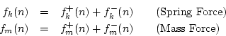
- ... complementary|textbf.7.1
- To show this, let
 denote the reflection transfer function (``reflectance'') of the bell
for pressure waves, and
denote the reflection transfer function (``reflectance'') of the bell
for pressure waves, and  the transmission transfer function
(``transmittance''). Then, as discussed in §K.2 and
§G.8, linearity and energy conservation demand that
for pressure waves, and
for velocity waves. (For velocity waves, the transmittance is
, while the reflectance is
the transmission transfer function
(``transmittance''). Then, as discussed in §K.2 and
§G.8, linearity and energy conservation demand that
for pressure waves, and
for velocity waves. (For velocity waves, the transmittance is
, while the reflectance is  .) Thus, the sum of
transmitted and reflected power at frequency
.) Thus, the sum of
transmitted and reflected power at frequency  is
where
is
where  denotes the z transform of the pressure signal transmitted
through the bell, and
denotes the z transform of the pressure signal transmitted
through the bell, and  denotes the reflected pressure wave.
Similarly,
denotes the reflected pressure wave.
Similarly,  and
and  denote the transmitted and reflected
velocity waves (
denote the transmitted and reflected
velocity waves ( flips the reflected velocity wave to that it
flows in the same direction as the transmitted velocity wave), and
flips the reflected velocity wave to that it
flows in the same direction as the transmitted velocity wave), and  and
and  denote the pressure and velocity waves incident on the
bell. All of these z transform have omitted arguments
denote the pressure and velocity waves incident on the
bell. All of these z transform have omitted arguments
 ,
where denotes the sampling interval in seconds.
,
where denotes the sampling interval in seconds.
.
.
.
.
.
.
.
.
.
.
.
.
.
.
.
.
.
.
.
.
.
.
.
.
.
.
.
.
.
.
- ...
closure.7.2
- For operation in fixed-point DSP chips, the
independent variable
 is generally confined to the interval
  . Note that having the
table go all the way to zero at the maximum negative pressure
. Note that having the
table go all the way to zero at the maximum negative pressure
 is not physically reasonable (0.8 would be more reasonable), but it has the
practical benefit that when the lookup-table input signal is about to clip,
the reflection coefficient goes to zero, thereby opening the feedback
loop.
is not physically reasonable (0.8 would be more reasonable), but it has the
practical benefit that when the lookup-table input signal is about to clip,
the reflection coefficient goes to zero, thereby opening the feedback
loop.
.
.
.
.
.
.
.
.
.
.
.
.
.
.
.
.
.
.
.
.
.
.
.
.
.
.
.
.
.
.
- ...exponentially9.1
- If the flare of the bell is expressed as
 , where
  denotes the horn radius at
position along the bore axis, then
denotes the horn radius at
position along the bore axis, then  is called the
flare constant of the bell.
is called the
flare constant of the bell.
.
.
.
.
.
.
.
.
.
.
.
.
.
.
.
.
.
.
.
.
.
.
.
.
.
.
.
.
.
.
- ... pressure9.2
- As always
in this book, by ``air pressure'' we mean the excess air
pressure above ambient air pressure. In the case of brass
instruments, excess air pressure is created by the muscles of the
lungs.
.
.
.
.
.
.
.
.
.
.
.
.
.
.
.
.
.
.
.
.
.
.
.
.
.
.
.
.
.
.
- ... mouthpiece.9.3
- When
the kinetic energy of a jet is converted back into air pressure, this
is called pressure recovery. We assume, following
[92] and others, that pressure recovery does not occur
in this model. Instead, the kinetic energy of the ket is assumed to
be dissipated in the form of turbulence (vortices and ultimately
heat). Note that air flow is therefore assumed inviscid within the
mouth and between the lips, but viscous around the jet in the
mouthpiece.
.
.
.
.
.
.
.
.
.
.
.
.
.
.
.
.
.
.
.
.
.
.
.
.
.
.
.
.
.
.
- ...Putland.9.4
- For velocity waves, the flare may be
hyperbolic [45].
.
.
.
.
.
.
.
.
.
.
.
.
.
.
.
.
.
.
.
.
.
.
.
.
.
.
.
.
.
.
- ...
below).A.1
- A shorter method for unzipping and unpacking is
zcat delay.tar.gz | tar -xvf -
.
.
.
.
.
.
.
.
.
.
.
.
.
.
.
.
.
.
.
.
.
.
.
.
.
.
.
.
.
.
- ...MakefilesA.2
- Only STK makefiles are regenerated by
configure--the files
myproj/Makefile
and
myproj/Makefile.proj
must be edited by hand, if needed.
.
.
.
.
.
.
.
.
.
.
.
.
.
.
.
.
.
.
.
.
.
.
.
.
.
.
.
.
.
.
- ...
option.A.3
- If you encounter any ``missing statements'' or variables while
single-stepping gdb, try turning optimization off
altogether by removing the -O2 option from CFLAGS in the
Makefile.
.
.
.
.
.
.
.
.
.
.
.
.
.
.
.
.
.
.
.
.
.
.
.
.
.
.
.
.
.
.
- ... <Enter>.A.4
- The notation M-x,
pronounced ``meta x,'' means to hold down the Alt key and press
the x key. Alternatively, one can type the Esc key
followed by the x key. In either case, emacs
will prompt for a command line input. The notation <Enter>
means, of course, the Enter key (sometimes labeled
Return).
.
.
.
.
.
.
.
.
.
.
.
.
.
.
.
.
.
.
.
.
.
.
.
.
.
.
.
.
.
.
- ... below.B.1
- For further introductory information
regarding compiling, linking, and debugging programs in the UNIX
environment, see http://cslibrary.stanford.edu/107/.
.
.
.
.
.
.
.
.
.
.
.
.
.
.
.
.
.
.
.
.
.
.
.
.
.
.
.
.
.
.
- ... folder).B.2
- It is good practice to use your own
folder, e.g., myprojects instead of
projects, so that you can simply copy myprojects
into new releases of the STK (and start debugging all over again -
 ).
).
.
.
.
.
.
.
.
.
.
.
.
.
.
.
.
.
.
.
.
.
.
.
.
.
.
.
.
.
.
.
- ... messageC.1
- In C++, ``sending message to object ''
amounts simply to executing function in struct . This is
sometimes referred to static binding, as opposed to
dynamic binding.
.
.
.
.
.
.
.
.
.
.
.
.
.
.
.
.
.
.
.
.
.
.
.
.
.
.
.
.
.
.
- ...dAlembert.D.1
- For a short biography of d'Alembert, see
http:
//www-groups.dcs.st-and.ac.uk/~history/Mathematicians/D'Alembert.html
.
.
.
.
.
.
.
.
.
.
.
.
.
.
.
.
.
.
.
.
.
.
.
.
.
.
.
.
.
.
- ... (1685-1731)D.2
- http:
//<ibidem>/Taylor.html
.
.
.
.
.
.
.
.
.
.
.
.
.
.
.
.
.
.
.
.
.
.
.
.
.
.
.
.
.
.
- ... (1707-1783)D.3
- http:
//<ibidem>/Euler.html
.
.
.
.
.
.
.
.
.
.
.
.
.
.
.
.
.
.
.
.
.
.
.
.
.
.
.
.
.
.
- ...
eyeglasses.D.4
- http://www.mathphysics.com/pde/history.html
.
.
.
.
.
.
.
.
.
.
.
.
.
.
.
.
.
.
.
.
.
.
.
.
.
.
.
.
.
.
- ... vibrations.D.5
- http:
//www.stetson.edu/~efriedma/periodictable/html/B.html
.
.
.
.
.
.
.
.
.
.
.
.
.
.
.
.
.
.
.
.
.
.
.
.
.
.
.
.
.
.
- ...ZadehAndDesoer,Kailath80,Depalle.D.6
- http://ccrma.stanford.edu/~jos/PianoString/
.
.
.
.
.
.
.
.
.
.
.
.
.
.
.
.
.
.
.
.
.
.
.
.
.
.
.
.
.
.
- ...strain.D.7
- http://www.efunda.com/formulae/solid_mechanics/mat_mechanics/hooke.cfm
.
.
.
.
.
.
.
.
.
.
.
.
.
.
.
.
.
.
.
.
.
.
.
.
.
.
.
.
.
.
- ...
public.D.8
- http:
//cnx.rice.edu/content/m0050/latest/
.
.
.
.
.
.
.
.
.
.
.
.
.
.
.
.
.
.
.
.
.
.
.
.
.
.
.
.
.
.
- ...FettweisMain.D.9
- Derivation:
http://ccrma.stanford.edu/~jos/pasp/Wave_Digital_Filters.html
.
.
.
.
.
.
.
.
.
.
.
.
.
.
.
.
.
.
.
.
.
.
.
.
.
.
.
.
.
.
- ...
Belevitch.D.10
- http://www.ieee.org/organizations/history_center/oral_histories/transcripts/fettweis.html
.
.
.
.
.
.
.
.
.
.
.
.
.
.
.
.
.
.
.
.
.
.
.
.
.
.
.
.
.
.
- ...Flanagan72,FlanaganAndRabinerEds,RabinerAndSchafer78,SchaferAndMarkel79,OShaughnessy87,DPH93,Keller94.D.11
- The
overview [285] of early speech production models is
freely available online, thanks to the Smithsonian Speech Synthesis
History Project.
.
.
.
.
.
.
.
.
.
.
.
.
.
.
.
.
.
.
.
.
.
.
.
.
.
.
.
.
.
.
- ... formulation.D.12
- http:
en.wikipedia.org/wiki/Oliver_Heaviside
.
.
.
.
.
.
.
.
.
.
.
.
.
.
.
.
.
.
.
.
.
.
.
.
.
.
.
.
.
.
- ... phenomenon.D.13
- http:www.microwaves101.com/encyclopedia/history.cfm
.
.
.
.
.
.
.
.
.
.
.
.
.
.
.
.
.
.
.
.
.
.
.
.
.
.
.
.
.
.
- ...D.14
- Scattering
theory:
http://ccrma.stanford.edu/~jos/pasp/Scattering_Impedance_Changes.html
.
.
.
.
.
.
.
.
.
.
.
.
.
.
.
.
.
.
.
.
.
.
.
.
.
.
.
.
.
.
- ... method.D.15
- ``Bicycle Built for
Two'' by Kelly, Lochbaum, and Matthews,
1961:
http://ccrma.stanford.edu/~jos/wav/daisy-klm.wav
.
.
.
.
.
.
.
.
.
.
.
.
.
.
.
.
.
.
.
.
.
.
.
.
.
.
.
.
.
.
- ... completion.D.16
- http://www.bell-labs.com/news/1997/march/5/2.html
.
.
.
.
.
.
.
.
.
.
.
.
.
.
.
.
.
.
.
.
.
.
.
.
.
.
.
.
.
.
- ...PRCT.D.17
- http:
www.cs.princeton.edu/~prc/SingingSynth.html (includes sound
examples)
.
.
.
.
.
.
.
.
.
.
.
.
.
.
.
.
.
.
.
.
.
.
.
.
.
.
.
.
.
.
- ...SchellengA,SchellengB,CremerC.D.18
- http://www.zainea.com/Oscilationsofbowedstring.htm
.
.
.
.
.
.
.
.
.
.
.
.
.
.
.
.
.
.
.
.
.
.
.
.
.
.
.
.
.
.
- ...
simpleE.1
- While this formula seems fairly simple now, in
Newton's day, it was necessary to invent calculus before it
could be stated in this way.
.
.
.
.
.
.
.
.
.
.
.
.
.
.
.
.
.
.
.
.
.
.
.
.
.
.
.
.
.
.
- ... velocity.E.2
- The only
massless particles are the photon and graviton (presuming it exists),
and massless particles can only travel at the speed of light. By
Einstein's famous formula
 , we know that a particle's mass is
proportional to its energy at rest.
, we know that a particle's mass is
proportional to its energy at rest.
.
.
.
.
.
.
.
.
.
.
.
.
.
.
.
.
.
.
.
.
.
.
.
.
.
.
.
.
.
.
- ...
constant|textbf.E.3
- The gravitation constant is given in
International Standard Units (``SI units'')
by
where the following physical units abbreviations are used:
These physical units for  come directly from Newton's second law of
motion (§E.1).
come directly from Newton's second law of
motion (§E.1).
.
.
.
.
.
.
.
.
.
.
.
.
.
.
.
.
.
.
.
.
.
.
.
.
.
.
.
.
.
.
- ...force|textbf.E.4
- From
a modern point of view, all forces are ``mediated'' by some particle,
and there are only four basic forces: The electromagnetic force
is mediated by the photon, the
strong nuclear force is mediated
by the gluon, the weak nuclear force is mediated the
 and
and  bosons, and gravity is thought to be mediated by
the graviton, although gravity is not yet incorporated into the
Standard Model of theoretical physics. Only the electromagnetic
and gravitational forces are encountered in everyday life, since the
strong and weak nuclear forces decay exponentially on the scale of an
atomic nucleus. The approximate relative strengths of the
strong:weak:EM:gravity forces are
bosons, and gravity is thought to be mediated by
the graviton, although gravity is not yet incorporated into the
Standard Model of theoretical physics. Only the electromagnetic
and gravitational forces are encountered in everyday life, since the
strong and weak nuclear forces decay exponentially on the scale of an
atomic nucleus. The approximate relative strengths of the
strong:weak:EM:gravity forces are
 . At very high
energies, the weak and EM forces unify, according to the Standard
Model.
. At very high
energies, the weak and EM forces unify, according to the Standard
Model.
.
.
.
.
.
.
.
.
.
.
.
.
.
.
.
.
.
.
.
.
.
.
.
.
.
.
.
.
.
.
- ... force.E.5
- In this example, the
mass-spring system is in
equilibrium (not moving), so all forces in the system must sum
to zero. Equilibrium also must hold if the whole system is traveling
with a constant velocity; in other words, it is the lack of
relative motion that matters.
.
.
.
.
.
.
.
.
.
.
.
.
.
.
.
.
.
.
.
.
.
.
.
.
.
.
.
.
.
.
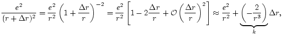
- ... displacements.E.6
- To show
this quantitatively, consider two electrons, each having electric
charge
 , separated by
  meters. Then the Coulomb force between
the electrons is proportional to
meters. Then the Coulomb force between
the electrons is proportional to  . Adding a small
perturbation
. Adding a small
perturbation  to yields a new force proportional to
where we used the binomial expansion to obtain the
approximation. (The notation
to yields a new force proportional to
where we used the binomial expansion to obtain the
approximation. (The notation
 means ``terms order
of
means ``terms order
of
 '', and such terms approach zero as fast as
approaches zero.) Thus, the effective spring constant
connecting the two electrons is
'', and such terms approach zero as fast as
approaches zero.) Thus, the effective spring constant
connecting the two electrons is  , when
 .
.
.
.
.
.
.
.
.
.
.
.
.
.
.
.
.
.
.
.
.
.
.
.
.
.
.
.
.
.
.
.
- ... yieldingE.7
- A more formal methodology for arriving
at differential equations by applying Newton's law and Hooke's law is
described in Appendix N. In the present example, consideration of the
underlying physics should convince you that the signs in Eq. (E.4)
are correct. For example, when is positive, the spring must push
the mass back to the left. Therefore,
 means the mass
will be accelerated to the left.
means the mass
will be accelerated to the left.
.
.
.
.
.
.
.
.
.
.
.
.
.
.
.
.
.
.
.
.
.
.
.
.
.
.
.
.
.
.
- ...
time:E.8
- See, e.g.,
[426, p. 235-236] for a derivation, and Appendix N,
specifically §N.3.6, for related analysis.
.
.
.
.
.
.
.
.
.
.
.
.
.
.
.
.
.
.
.
.
.
.
.
.
.
.
.
.
.
.
- ...
object.E.9
- In SI units, work is in units called
Joules (abbreviated J).
Thus, Joules are Newtons times meters.
.
.
.
.
.
.
.
.
.
.
.
.
.
.
.
.
.
.
.
.
.
.
.
.
.
.
.
.
.
.
- ... considered.E.10
- Ok, there does exist energy
fluctuation on the scale of ``Heisenberg uncertainty''. That is, it
is possible to have a violation in energy conservation by an amount
 over a time duration
  , provided
 is sufficiently small (on the order of Planck's constant
  ).
This can be considered a form of the Heisenberg uncertainty principle.
).
This can be considered a form of the Heisenberg uncertainty principle.
.
.
.
.
.
.
.
.
.
.
.
.
.
.
.
.
.
.
.
.
.
.
.
.
.
.
.
.
.
.
- ... potential:E.11
- This was first pointed out
by Rayleigh [327, p. 39].
.
.
.
.
.
.
.
.
.
.
.
.
.
.
.
.
.
.
.
.
.
.
.
.
.
.
.
.
.
.
- ... gases:E.12
-
http://www.grc.nasa.gov/WWW/K-12/airplane/sound.html
.
.
.
.
.
.
.
.
.
.
.
.
.
.
.
.
.
.
.
.
.
.
.
.
.
.
.
.
.
.
- ...G.1
- Any function of
 , where denotes time and denotes
position along a ``waveshape'', may be interpreted as a fixed
waveshape traveling to the right (positive direction), with
speed
, where denotes time and denotes
position along a ``waveshape'', may be interpreted as a fixed
waveshape traveling to the right (positive direction), with
speed  . Similarly, any function of
  may be seen as a
waveshape traveling to the left (negative direction) at
speed meters per second. In both cases, denotes a position
along the waveshape, and denotes time. For any fixed , a
``snapshot'' of the waveshape may be seen by evaluating along .
may be seen as a
waveshape traveling to the left (negative direction) at
speed meters per second. In both cases, denotes a position
along the waveshape, and denotes time. For any fixed , a
``snapshot'' of the waveshape may be seen by evaluating along .
.
.
.
.
.
.
.
.
.
.
.
.
.
.
.
.
.
.
.
.
.
.
.
.
.
.
.
.
.
.
- ... velocity|textbfG.2
- The term
phase velocity is normally used when it differs
from the group velocity, as in stiff, dispersive strings
(§G.6).
In the present context, the phase velocity and group velocity are
the same, so the term ``wave velocity'' is unambigous here.
See the analogous terms phase delay and group delay
in [426] for more details about the difference.
.
.
.
.
.
.
.
.
.
.
.
.
.
.
.
.
.
.
.
.
.
.
.
.
.
.
.
.
.
.
- ...
scattering.G.3
- Here it is assumed that
 and
and  in
the Kelly-Lochbaum junction can be computed exactly from
in
the Kelly-Lochbaum junction can be computed exactly from  in the
number system being used. This is the case in two's complement
arithmetic as is typically used in practice.
in the
number system being used. This is the case in two's complement
arithmetic as is typically used in practice.
.
.
.
.
.
.
.
.
.
.
.
.
.
.
.
.
.
.
.
.
.
.
.
.
.
.
.
.
.
.
- ...
``right-going.''G.4
- In the acoustic tube literature which
involves only a cascade chain of acoustic waveguides,
 is
taken to be traveling to the right along the axis of the tube
[275]. In classical network theory [33] and in
circuit theory, velocity (current) at the terminals of an -port
device is by convention taken to be positive when it flows into
the device.
is
taken to be traveling to the right along the axis of the tube
[275]. In classical network theory [33] and in
circuit theory, velocity (current) at the terminals of an -port
device is by convention taken to be positive when it flows into
the device.
.
.
.
.
.
.
.
.
.
.
.
.
.
.
.
.
.
.
.
.
.
.
.
.
.
.
.
.
.
.
- ... foundG.5
- http://ccrma.stanford.edu/~jos/filters/Similarity_Transformations.html
.
.
.
.
.
.
.
.
.
.
.
.
.
.
.
.
.
.
.
.
.
.
.
.
.
.
.
.
.
.
- ... magnitude:G.6
- While the
literature seems to mention this property only for prime numbers
 ,
it is straightforward to show that it holds in fact for all positive odd
integers . Prime values of have advantages, however, when harmonics
of the ``design frequency'' are considered.
,
it is straightforward to show that it holds in fact for all positive odd
integers . Prime values of have advantages, however, when harmonics
of the ``design frequency'' are considered.
.
.
.
.
.
.
.
.
.
.
.
.
.
.
.
.
.
.
.
.
.
.
.
.
.
.
.
.
.
.
- ... samples.I.1
- Classically, an interpolation
 of discrete data points
  always required
 ;
that is, the interpolating function must always pass through the given
data points. More recently, however, particularly in the field of
computer graphics, interpolation schemes such as Bezier splines
have been defined which do not always pass through the known points.
;
that is, the interpolating function must always pass through the given
data points. More recently, however, particularly in the field of
computer graphics, interpolation schemes such as Bezier splines
have been defined which do not always pass through the known points.
.
.
.
.
.
.
.
.
.
.
.
.
.
.
.
.
.
.
.
.
.
.
.
.
.
.
.
.
.
.
- ....I.2
- Of course, all derivatives of must
be calculated from the underlying continuous signal
 represented by the samples and then evaluated at
  .
.
.
.
.
.
.
.
.
.
.
.
.
.
.
.
.
.
.
.
.
.
.
.
.
.
.
.
.
.
.
.
- ...JOSFP.I.3
- To see this, note that the integral of the
group delay around the unit circle is simply minus the winding
number of the phase response (the number of zeros minus the number of
poles inside the unit circle):
By the graphical method for phase response calculation [426, Chapter
8], each zero contributes
 radians to
 , and each pole contributes
  radians. Thus,
the average group delay around the unit circle is
radians. Thus,
the average group delay around the unit circle is
.
.
.
.
.
.
.
.
.
.
.
.
.
.
.
.
.
.
.
.
.
.
.
.
.
.
.
.
.
.
- ... kHz.I.4
- We arbitrarily define the
 % guard band as a
percentage of half the sampling rate actually used, not as % of the
desired kHz bandwidth which would call for a
% guard band as a
percentage of half the sampling rate actually used, not as % of the
desired kHz bandwidth which would call for a  kHz sampling rate.
.
.
.
.
.
.
.
.
.
.
.
.
.
.
.
.
.
.
.
.
.
.
.
.
.
.
.
.
.
.
- ... transform|textbf,J.1
- For a short online introduction to Laplace transforms, see, e.g.,
http://ccrma.stanford.edu/~jos/filters/Laplace_Transform_Analysis.html.
.
.
.
.
.
.
.
.
.
.
.
.
.
.
.
.
.
.
.
.
.
.
.
.
.
.
.
.
.
.
- ... mass.''J.2
- We say that the driving point of every mechanical
system must ``looks like a mass'' at sufficiently high frequency
because every mechanical system has at least some mass, and the
driving-point impedance of a mass goes to infinity with frequency.
However, in a completely detailed model, the contact force between
objects should really be the Coulombe force, which ``looks like
a spring''. In other words, mechanical interactions are ultimately
electromagnetic interactions, and it is theoretically possible for a
driving force on an atom to be so small and fast that it can vibrate
the outermost electron orbital without moving the nucleus appreciably,
thus ``looking like a spring'' in the high-frequency limit. We will
not be concerned with atomic-scale models in this book, and will
persist in treating masses and springs in idealized form.
.
.
.
.
.
.
.
.
.
.
.
.
.
.
.
.
.
.
.
.
.
.
.
.
.
.
.
.
.
.
- ....J.3
- To avoid the introduction of
half a sample of delay by the approximation, the first-order finite
difference may be defined instead as
![$ x[(n+1)T]-x[(n-1)T]/(2T)$](img2498.png) .
.
.
.
.
.
.
.
.
.
.
.
.
.
.
.
.
.
.
.
.
.
.
.
.
.
.
.
.
.
.
.
- ....J.4
- Note that the
matched transformation would be more precisely scaled if it were
defined as
This can be seen by taking the first-order Taylor series expansion of
the right-hand side. (It also makes more sense in terms of physical
units.) However, scale factors are very often dropped.
.
.
.
.
.
.
.
.
.
.
.
.
.
.
.
.
.
.
.
.
.
.
.
.
.
.
.
.
.
.
- ... case.J.5
- In the
case of complex impedances, the matched impedance case becomes
 .
.
.
.
.
.
.
.
.
.
.
.
.
.
.
.
.
.
.
.
.
.
.
.
.
.
.
.
.
.
.
.
- ... output.K.1
- So-called
``electric-acoustic'' guitars, such as the Godin electric-acoustic,
use piezoelectric crystals in the bridge to measure string force at
the string endpoint. Electric violins, such as the Zeta Violin,
typically use this approach as well.
.
.
.
.
.
.
.
.
.
.
.
.
.
.
.
.
.
.
.
.
.
.
.
.
.
.
.
.
.
.
- ... measurements,K.2
- The Matlab function
cohere() can be used to compute the coherence function
between two sampled spectra.
.
.
.
.
.
.
.
.
.
.
.
.
.
.
.
.
.
.
.
.
.
.
.
.
.
.
.
.
.
.
- ... phase.K.3
- Zero-phase filters can normally be
implemented in practice because there are pure delay lines preceding and
following the reflectance filter, and taps can be introduced in the
delay-line preceding the reflectance to implement noncausal terms in the
impulse response.
.
.
.
.
.
.
.
.
.
.
.
.
.
.
.
.
.
.
.
.
.
.
.
.
.
.
.
.
.
.
- ....K.4
- To
prove this, note that the roots of
 are the reciprocals of the
roots of
are the reciprocals of the
roots of  , since the conformal map
 exchanges
interior of the unit circle with the exterior of the unit circle.
exchanges
interior of the unit circle with the exterior of the unit circle.
.
.
.
.
.
.
.
.
.
.
.
.
.
.
.
.
.
.
.
.
.
.
.
.
.
.
.
.
.
.
- ...
disk.K.5
- The strict outer disk is defined as the region
 in the extended complex plane.
.
.
.
.
.
.
.
.
.
.
.
.
.
.
.
.
.
.
.
.
.
.
.
.
.
.
.
.
.
.
- ... wave.N.1
- When there are more than two
ports at a junction, the `
 ' superscript will denote a wave
traveling into the junction.
' superscript will denote a wave
traveling into the junction.
.
.
.
.
.
.
.
.
.
.
.
.
.
.
.
.
.
.
.
.
.
.
.
.
.
.
.
.
.
.
- ... network.N.2
- Wave
digital filters are not the same thing as digital waveguide networks,
however, because the wave variables in a wave digital filter have a
compressed frequency spectrum (from the bilinear transform), while the
signals in a digital waveguide network have a bandlimited spectrum
which is not warped.
.
.
.
.
.
.
.
.
.
.
.
.
.
.
.
.
.
.
.
.
.
.
.
.
.
.
.
.
.
.
- ...
waveguideN.3
- Here, it is perhaps most concrete to think in terms
of electrical equivalent circuits, so that the mass is an inductor and
a ``waveguide'' is a ``transmission line.''
.
.
.
.
.
.
.
.
.
.
.
.
.
.
.
.
.
.
.
.
.
.
.
.
.
.
.
.
.
.
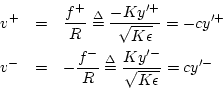
- ... mass,N.4
- The phase delay,
for example, of the reflectance
 of an ideal spring is
given by
At
of an ideal spring is
given by
At  rad/sec, in particular,
the phase delay is
rad/sec, in particular,
the phase delay is
![$ P(1)=-\angle[(1-j)/(1+j)]=-\angle(-j) = \pi/2$](img3339.png) .
Since the period is when , this is a quarter-cycle
of delay.
.
Since the period is when , this is a quarter-cycle
of delay.
After the bilinear transform
 , the phase delay becomes
where  is defined by
 (the
relationship between continuous-time frequency and discrete-time
frequency imposed by the bilinear transform). Thus, the phase delay
comes out to exactly one sample at each frequency. Checking the point
(the
relationship between continuous-time frequency and discrete-time
frequency imposed by the bilinear transform). Thus, the phase delay
comes out to exactly one sample at each frequency. Checking the point
 ,
i.e., four samples per period, we find that one sample of delay does
in fact correspond to a quarter-cycle of delay.
,
i.e., four samples per period, we find that one sample of delay does
in fact correspond to a quarter-cycle of delay.
The same holds true for the group delay of the spring reflectance:
We see that the frequency-warping under the bilinear transform serves
to move each frequency to the unique point along the unit circle at
which the reflectance of a mass or spring happens to be exactly one
sample. The mass reflectance additionally inverts.
.
.
.
.
.
.
.
.
.
.
.
.
.
.
.
.
.
.
.
.
.
.
.
.
.
.
.
.
.
.
- ...tankwdf.N.5
- Note that the wave
variables are now labeled in element-centric notation as opposed to
adaptor-centric notation:
.
.
.
.
.
.
.
.
.
.
.
.
.
.
.
.
.
.
.
.
.
.
.
.
.
.
.
.
.
.
- ... limit.N.6
- Note that the mass and
velocity limits are tied together such that
 constant. This
information is lost in the final limits because the expression
constant. This
information is lost in the final limits because the expression
 is ``indeterminate''.
.
.
.
.
.
.
.
.
.
.
.
.
.
.
.
.
.
.
.
.
.
.
.
.
.
.
.
.
.
.
- ...
algorithms.O.1
- See [97] for discussion of a wider
variety of digital sine generation methods.
.
.
.
.
.
.
.
.
.
.
.
.
.
.
.
.
.
.
.
.
.
.
.
.
.
.
.
.
.
.
- ... algorithm,O.2
- The
``magic circle'' algorithm is so named because it generates closed
curves in the
 plane even when numerical precision is
very low. For this reason, it has long been used as an algorithm
for drawing ``circles'' (actually ellipses) in computer graphics.
The algorithm is derived naturally by numerically integrating the
derivative relationships between sine and cosine:
plane even when numerical precision is
very low. For this reason, it has long been used as an algorithm
for drawing ``circles'' (actually ellipses) in computer graphics.
The algorithm is derived naturally by numerically integrating the
derivative relationships between sine and cosine:
.
.
.
.
.
.
.
.
.
.
.
.
.
.
.
.
.
.
.
.
.
.
.
.
.
.
.
.
.
.
- ...
amplitude),O.3
- When
 is constant, the time constant
 of the ensuing exponential growth or decay may be found by
solving
of the ensuing exponential growth or decay may be found by
solving
 for to obtain
 ln
ln , where
denotes the sampling interval, and
ln denotes the natural
logarithm of .
, where
denotes the sampling interval, and
ln denotes the natural
logarithm of .
.
.
.
.
.
.
.
.
.
.
.
.
.
.
.
.
.
.
.
.
.
.
.
.
.
.
.
.
.
.
- ... analysisO.4
- http://ccrma.stanford.edu/~jos/filters/State_Space_Models.html
.
.
.
.
.
.
.
.
.
.
.
.
.
.
.
.
.
.
.
.
.
.
.
.
.
.
.
.
.
.
- ... modeling,P.1
- The
general field in which transfer function descriptions are estimated
for physical systems is called ``system identification''
[268,404], and it is used extensively in industrial
automatic control applications.
.
.
.
.
.
.
.
.
.
.
.
.
.
.
.
.
.
.
.
.
.
.
.
.
.
.
.
.
.
.
- ....P.2
- For convenience, we typically define the
discrete-time counterpart of a continuous-time function as though the
sampling interval were
 .
.
.
.
.
.
.
.
.
.
.
.
.
.
.
.
.
.
.
.
.
.
.
.
.
.
.
.
.
.
.
.
- ...SmithCommutedFromPASP,MattiGuitar,MattiAndSmith96.Q.1
- Extracts of
this material were published previously in [213].
.
.
.
.
.
.
.
.
.
.
.
.
.
.
.
.
.
.
.
.
.
.
.
.
.
.
.
.
.
.
- ... volume.Q.2
- These remarks apply to playback of the
excitation only. The string provides further filtering which could be
taken into account. However, to a first approximation, the string
filtering is like a ``sampling'' of the excitation spectrum, with a
gentle roll-off at high frequencies due to the lowpass loop
filtering. Also, the string is a highly variable filter with many
settings. It is therefore reasonable to ignore the string filtering
when determining an optimal preemphasis for excitation-table
quantization.
.
.
.
.
.
.
.
.
.
.
.
.
.
.
.
.
.
.
.
.
.
.
.
.
.
.
.
.
.
.
- ... parts.R.1
- It is not necessary to
perform a Taylor series expansion to separate out the even and odd
parts of a function. Instead, the even part of can be computed
as
![$ f_e(x) = [f(x)+f(-x)]/2$](img3669.png) and the odd part as
and the odd part as
![$ f_o(x) =
[f(x)-f(-x)]/2$](img3670.png) . It is easily checked that
. It is easily checked that  is even,
  is
odd, and
is
odd, and  .
.
.
.
.
.
.
.
.
.
.
.
.
.
.
.
.
.
.
.
.
.
.
.
.
.
.
.
.
.
.
.
- ... mapping.R.2
- Note that
memoryless nonlinearities used for distortion simulation are typically
odd functions of instantaneous amplitude, such as
 . (A good practical choice is given in
Eq. (R.3).) However, in guitar-amplifier distortion
simulation, even-order terms are considered quite important
[367].
. (A good practical choice is given in
Eq. (R.3).) However, in guitar-amplifier distortion
simulation, even-order terms are considered quite important
[367].
.
.
.
.
.
.
.
.
.
.
.
.
.
.
.
.
.
.
.
.
.
.
.
.
.
.
.
.
.
.
- ...R.3
- The convolution theorem for Fourier transforms states that
convolution in the time domain corresponds to pointwise multiplication
in the frequency domain [426]. The dual of the convolution
theorem states just the opposite: Pointwise multiplication in the time
domain corresponds to convolution in the frequency domain. Thus, if
the spectrum of is
 , then the spectrum of
  is
is
 , where ``
 '' denotes the convolution
operation.
'' denotes the convolution
operation.
.
.
.
.
.
.
.
.
.
.
.
.
.
.
.
.
.
.
.
.
.
.
.
.
.
.
.
.
.
.
- ... spectra.R.4
- The
basilar membrane of the ear (which is rolled up inside the
snail-shaped cochlea of the ear) effectively performs a real-time
Fourier analysis which is ``felt'' by nerve cells leading to the
brain.
.
.
.
.
.
.
.
.
.
.
.
.
.
.
.
.
.
.
.
.
.
.
.
.
.
.
.
.
.
.
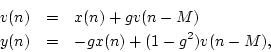
![$\displaystyle \mathbf{H}_4 \isdef
\frac{1}{\sqrt{2}}
\left[\begin{array}{rr}
\...
...}{rrrr}
1& 1& 1&1\\
-1& 1&-1&1\\
-1&-1& 1&1\\
1&-1&-1&1
\end{array}\right].
$](img425.png)