 |
The FDN can be seen as a vector feedback comb filter,2.6obtained by replacing the delay line with a diagonal delay matrix
(defined in Eq. (1.10) below), and replacing the feedback gain
![]() by the product of a diagonal matrix
by the product of a diagonal matrix
![]() times an orthogonal
matrix
times an orthogonal
matrix
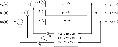
![]() , as shown in
Fig. 1.22 for
, as shown in
Fig. 1.22 for ![]() . The time-update for this FDN can be written
as
. The time-update for this FDN can be written
as
![$\displaystyle \left[\begin{array}{c} y_1(n) \\ [2pt] y_2(n) \\ [2pt] y_3(n)\end...
...array}{c} x_1(n-M_1) \\ [2pt] x_2(n-M_2) \\ [2pt] x_3(n-M_3)\end{array}\right],$](img248.png) |
(2.7) |
| (2.8) | |||
| (2.9) |
![$\displaystyle \left[\begin{array}{c} x_1(n) \\ [2pt] x_2(n) \\ [2pt] x_3(n)\end...
...gin{array}{c} u_1(n) \\ [2pt] u_2(n) \\ [2pt] u_3(n)\end{array}\right] \protect$](img247.png)
![$\displaystyle \mathbf{D}(z) \isdef \left[\begin{array}{ccc} z^{-M_1} & 0 & 0\\ [2pt] 0 & z^{-M_2} & 0\\ [2pt] 0 & 0 & z^{-M_3} \end{array}\right]. \protect$](img254.png)