- ...1
- This section was added in the third printing of this book (September 2013).
.
.
.
.
.
.
.
.
.
.
.
.
.
.
.
.
.
.
.
.
.
.
.
.
.
.
.
.
.
.
- ...
email2
- jos at ccrma.stanford.edu
.
.
.
.
.
.
.
.
.
.
.
.
.
.
.
.
.
.
.
.
.
.
.
.
.
.
.
.
.
.
- ...
numbers.1.1
- Physicists and mathematicians use
 instead of
 to denote
  .
.
.
.
.
.
.
.
.
.
.
.
.
.
.
.
.
.
.
.
.
.
.
.
.
.
.
.
.
.
.
.
- ...
unknowns.2.1
- ``Linear'' in this context means that the unknowns
are multiplied only by constants--they may not be multiplied by each
other or raised to any power other than
 (e.g., not squared or cubed
or raised to the
(e.g., not squared or cubed
or raised to the  power). Linear systems of
  equations in
unknowns are very easy to solve compared to nonlinear systems
of
equations in
unknowns. For example, Matlab and Octave can
easily handle them. You learn all about this in a course on
Linear Algebra which is highly recommended for anyone
interested in getting involved with signal processing. Linear algebra
also teaches you all about matrices, which are introduced only
briefly in Appendix H.
equations in
unknowns are very easy to solve compared to nonlinear systems
of
equations in
unknowns. For example, Matlab and Octave can
easily handle them. You learn all about this in a course on
Linear Algebra which is highly recommended for anyone
interested in getting involved with signal processing. Linear algebra
also teaches you all about matrices, which are introduced only
briefly in Appendix H.
.
.
.
.
.
.
.
.
.
.
.
.
.
.
.
.
.
.
.
.
.
.
.
.
.
.
.
.
.
.
- ...
numbers2.2
- (multiplication, addition, division, distributivity
of multiplication over addition, commutativity of multiplication and
addition)
.
.
.
.
.
.
.
.
.
.
.
.
.
.
.
.
.
.
.
.
.
.
.
.
.
.
.
.
.
.
- ...field.2.3
- See, e.g.,
Eric Weisstein's World of Mathematics
(http://mathworld.wolfram.com/) for definitions of any
unfamiliar mathematical terms such as a field (which is described,
for example, at the easily guessed URL
http://mathworld.wolfram.com/Field.html).
.
.
.
.
.
.
.
.
.
.
.
.
.
.
.
.
.
.
.
.
.
.
.
.
.
.
.
.
.
.
- ... tool.2.4
- Proofs for the
fundamental theorem of algebra have a long history involving many of
the great names in classical mathematics. The first known rigorous
proof was by Gauss based on earlier efforts by Euler and Lagrange.
(Gauss also introduced the term ``complex number.'') An alternate
proof was given by Argand based on the ideas of d'Alembert. For a
summary of the history, see http://www-gap.dcs.st-and.ac.uk/~history/HistTopics/Fund_theorem_of_algebra.html
(the first Google search result for ``fundamental theorem of
algebra'' in July of 2002).
.
.
.
.
.
.
.
.
.
.
.
.
.
.
.
.
.
.
.
.
.
.
.
.
.
.
.
.
.
.
- ...3.1
- That the rationals are dense in the reals
is easy to show using decimal expansions. Let
 and
and  denote
any two distinct, positive, irrational real numbers. Since
and
are distinct, their decimal expansions must differ in some
digit, say the
denote
any two distinct, positive, irrational real numbers. Since
and
are distinct, their decimal expansions must differ in some
digit, say the  th. Without loss of generality, assume
  .
Form the rational number
.
Form the rational number  by zeroing all digits in the decimal
expansion of
after the
th. Then
by zeroing all digits in the decimal
expansion of
after the
th. Then
 , as needed.
For two negative real numbers, we can negate them, use the same
argument, and negate the result. For one positive and one negative
real number, the rational number zero lies between them.
, as needed.
For two negative real numbers, we can negate them, use the same
argument, and negate the result. For one positive and one negative
real number, the rational number zero lies between them.
.
.
.
.
.
.
.
.
.
.
.
.
.
.
.
.
.
.
.
.
.
.
.
.
.
.
.
.
.
.
- ... as3.2
- This was computed via N[Sqrt[2],60] in Mathematica.
Symbolic mathematics programs, such as Mathematica,
Maple (offered as a Matlab extension),
maxima (a free, GNU descendant of the original Macsyma,
written in Common Lisp, and available at
http://maxima.sourceforge.net),
GiNaC (the Maple-replacement
used in the Octave Symbolic Manipulation Toolbox),
or
Yacas (another free, open-source program with similar goals
as Mathematica), are handy tools for cranking out any number
of digits in irrational numbers such as
 . In
Yacas (as of Version 1.0.55), the syntax is
. In
Yacas (as of Version 1.0.55), the syntax is
Precision(60)
N(Sqrt(2))
Of course, symbolic math programs can do much more than this, such as
carrying out algebraic manipulations on polynomials and solving
systems of symbolic equations in closed form.
.
.
.
.
.
.
.
.
.
.
.
.
.
.
.
.
.
.
.
.
.
.
.
.
.
.
.
.
.
.
- ... rule,3.3
- We will use the chain rule from
calculus without proof. Note that the use of calculus is beyond the
normal level of this book. Since calculus is only needed at this one
point in the DFT-math story, the reader should not be discouraged if
its usage seems like ``magic''. Calculus will not be needed at all for
practical applications of the DFT, such as spectrum analysis,
discussed in Chapter 8.
.
.
.
.
.
.
.
.
.
.
.
.
.
.
.
.
.
.
.
.
.
.
.
.
.
.
.
.
.
.
- ....3.4
- Logarithms are reviewed in
Appendix F.
.
.
.
.
.
.
.
.
.
.
.
.
.
.
.
.
.
.
.
.
.
.
.
.
.
.
.
.
.
.
- ...
number3.5
- A number is said to be
transcendental if it is not a
root of any polynomial with integer coefficients, i.e., it is not an
algebraic number of any degree. (Rational numbers are algebraic
numbers of degree 1; irrational numbers include transcendental numbers
and algebraic numbers of degree greater than 1, such as
which is of degree 2.) See
http://mathworld.wolfram.com/TranscendentalNumber.html
for further discussion.
.
.
.
.
.
.
.
.
.
.
.
.
.
.
.
.
.
.
.
.
.
.
.
.
.
.
.
.
.
.
- ... by3.6
- In
Mathematica, the first 50 digits of
 may be computed by
the expression N[E,50] (``evaluate numerically the
reserved-constant E to 50 decimal places''). In the
Octave Symbolic Manipulation Toolbox (part of Octave Forge), one
may type ``digits(50); Exp(1)''.
may be computed by
the expression N[E,50] (``evaluate numerically the
reserved-constant E to 50 decimal places''). In the
Octave Symbolic Manipulation Toolbox (part of Octave Forge), one
may type ``digits(50); Exp(1)''.
.
.
.
.
.
.
.
.
.
.
.
.
.
.
.
.
.
.
.
.
.
.
.
.
.
.
.
.
.
.
- ...
unity.3.7
- Sometimes we see
 , which is
the complex conjugate of the definition we have used here. It is
similarly a primitive
, which is
the complex conjugate of the definition we have used here. It is
similarly a primitive  th root, since powers of it will generate all
other
th roots.
th root, since powers of it will generate all
other
th roots.
.
.
.
.
.
.
.
.
.
.
.
.
.
.
.
.
.
.
.
.
.
.
.
.
.
.
.
.
.
.
- ...
geo\-metry.3.8
- See, for example,
http://www-spof.gsfc.nasa.gov/stargaze/Strig5.htm.
.
.
.
.
.
.
.
.
.
.
.
.
.
.
.
.
.
.
.
.
.
.
.
.
.
.
.
.
.
.
- ... oscillator.4.1
- A mass-spring oscillator analysis is given at
http://ccrma.stanford.edu/~jos/filters/Mass_Spring_Oscillator_Analysis.html
(from the next book [71] in the music signal processing series).
.
.
.
.
.
.
.
.
.
.
.
.
.
.
.
.
.
.
.
.
.
.
.
.
.
.
.
.
.
.
- ... (LTI4.2
- A system
 is said to be
linear if for any two input signals
is said to be
linear if for any two input signals  and
and  , we have
![$ S[x_1(t) + x_2(t)] = S[x_1(t)] + S[x_2(t)]$](img404.png) . A system is said to be
time invariant if
. A system is said to be
time invariant if
![$ y(t)=S[x(t)]$](img405.png) implies
implies
![$ S[x(t-\tau)] = y(t-\tau)$](img406.png) . This subject is developed in detail in
the second book [71] of the music signal processing series,
available on-line at
. This subject is developed in detail in
the second book [71] of the music signal processing series,
available on-line at
http://ccrma.stanford.edu/~jos/filters/.
.
.
.
.
.
.
.
.
.
.
.
.
.
.
.
.
.
.
.
.
.
.
.
.
.
.
.
.
.
.
- ...
soundfield,4.3
- For a definition, see
http://ccrma.stanford.edu/~jos/pasp/Mean_Free_Path.html
.
.
.
.
.
.
.
.
.
.
.
.
.
.
.
.
.
.
.
.
.
.
.
.
.
.
.
.
.
.
- ...combfilter.4.4
- Technically, Fig.4.3 shows the
feedforward comb filter, also called the ``inverse comb
filter'' [78]. The longer names are meant to
distinguish it from the feedback comb filter, in which the
delay output is fed back around the delay line and summed with
the delay input instead of the input being fed forward around
the delay line and summed with its output. (A diagram and further
discussion, including how time-varying comb filters create a
flanging effect, can be found at
http://ccrma.stanford.edu/~jos/pasp/Feedback_Comb_Filters.html.)
The frequency response of the feedforward comb filter is the inverse
of that of the feedback comb filter (one can cancel the effect of the
other), hence the name ``inverse comb filter.'' Frequency-response
analysis of digital filters is developed in [71] (available online).
.
.
.
.
.
.
.
.
.
.
.
.
.
.
.
.
.
.
.
.
.
.
.
.
.
.
.
.
.
.
- ... name.4.5
- While there is no reason it should be obvious
at this point, the comb-filter gain varies in fact sinusoidally
as a function of frequency.
.
.
.
.
.
.
.
.
.
.
.
.
.
.
.
.
.
.
.
.
.
.
.
.
.
.
.
.
.
.
- ...
dc4.6
- ``dc'' means ``direct current'' and is an electrical
engineering term for ``frequency 0
''.
.
.
.
.
.
.
.
.
.
.
.
.
.
.
.
.
.
.
.
.
.
.
.
.
.
.
.
.
.
.
- ... dB.4.7
- Recall that a gain factor
 is converted to decibels (dB) by the formula
 . See §F.2 for a review.
.
.
.
.
.
.
.
.
.
.
.
.
.
.
.
.
.
.
.
.
.
.
.
.
.
.
.
.
.
.
- ... receiver.4.8
- In practical AM radio,
single-sideband amplitude modulation is used, obtainable by filtering out the lower half of the spectrum we will
derive here, since it's not needed for broadcast.
.
.
.
.
.
.
.
.
.
.
.
.
.
.
.
.
.
.
.
.
.
.
.
.
.
.
.
.
.
.
- ...
practice.4.9
- An important variant of FM called
feedback FM, in which a single oscillator phase-modulates
itself, simply does not work if true frequency modulation is
implemented.
.
.
.
.
.
.
.
.
.
.
.
.
.
.
.
.
.
.
.
.
.
.
.
.
.
.
.
.
.
.
- ... section.4.10
- The mathematical derivation of FM
spectra is included here as a side note. No further use will be made
of it in this book.
.
.
.
.
.
.
.
.
.
.
.
.
.
.
.
.
.
.
.
.
.
.
.
.
.
.
.
.
.
.
- ...Watson44,4.11
- Existence of the
Laurent expansion follows from the fact that the generating function is a
product of an exponential function,
 , and an
exponential function inverted with respect to the unit circle,
, and an
exponential function inverted with respect to the unit circle,
 . It is readily verified by direct differentiation
in the complex plane that the exponential is an
entire function of
. It is readily verified by direct differentiation
in the complex plane that the exponential is an
entire function of  (analytic at all finite points in the complex
plane) [16], and therefore the inverted exponential is analytic
everywhere except at
(analytic at all finite points in the complex
plane) [16], and therefore the inverted exponential is analytic
everywhere except at  .
The desired Laurent expansion may be obtained, in principle,
by multiplying the one-sided series for the exponential and inverted exponential
together. The exponential series has the well known form
.
The desired Laurent expansion may be obtained, in principle,
by multiplying the one-sided series for the exponential and inverted exponential
together. The exponential series has the well known form
 . The series for the inverted exponential
can be obtained by inverting again (
. The series for the inverted exponential
can be obtained by inverting again (
 ), obtaining the
appropriate exponential series, and inverting each term.
), obtaining the
appropriate exponential series, and inverting each term.
.
.
.
.
.
.
.
.
.
.
.
.
.
.
.
.
.
.
.
.
.
.
.
.
.
.
.
.
.
.
- ...phasor),4.12
- Another example of phasor analysis can be found at
http://ccrma.stanford.edu/~jos/filters/Phasor_Analysis.html
(from the next book in this music signal processing series).
.
.
.
.
.
.
.
.
.
.
.
.
.
.
.
.
.
.
.
.
.
.
.
.
.
.
.
.
.
.
- ... signal|textbf.4.13
- In complex variables, a function
is ``analytic'' at a point
 if it is differentiable of
all orders at each point in some neighborhood of
if it is differentiable of
all orders at each point in some neighborhood of  [16]. Therefore, one might expect an ``analytic signal''
to be any signal which is differentiable of all orders at any point in
time, i.e., one that admits a fully valid Taylor expansion about any
point in time. However, all bandlimited signals (being sums of
finite-frequency sinusoids) are analytic in the complex-variables
sense at every point in time. Therefore, the signal processing term
``analytic signal'' refers instead to a signal having ``no negative
frequencies''. Equivalently, one could say that the spectrum of an analytic
signal is ``causal in the frequency domain''.
[16]. Therefore, one might expect an ``analytic signal''
to be any signal which is differentiable of all orders at any point in
time, i.e., one that admits a fully valid Taylor expansion about any
point in time. However, all bandlimited signals (being sums of
finite-frequency sinusoids) are analytic in the complex-variables
sense at every point in time. Therefore, the signal processing term
``analytic signal'' refers instead to a signal having ``no negative
frequencies''. Equivalently, one could say that the spectrum of an analytic
signal is ``causal in the frequency domain''.
.
.
.
.
.
.
.
.
.
.
.
.
.
.
.
.
.
.
.
.
.
.
.
.
.
.
.
.
.
.
- ... shift.4.14
- This operation is actually
used in some real-world AM and FM radio receivers (particularly in digital
radio receivers). The signal comes in centered about a high ``carrier
frequency'' (such as 101 MHz for radio station FM 101), so it looks very
much like a sinusoid at frequency 101 MHz. (The frequency modulation only
varies the carrier frequency in a relatively tiny interval about 101 MHz.
The total FM bandwidth including all the FM ``sidebands'' is about 100 kHz.
AM bands are only 10kHz wide.) By delaying the signal by 1/4 cycle, a good
approximation to the imaginary part of the analytic signal is created, and
its instantaneous amplitude and frequency are then simple to compute from
the analytic signal.
.
.
.
.
.
.
.
.
.
.
.
.
.
.
.
.
.
.
.
.
.
.
.
.
.
.
.
.
.
.
- ...demodulation4.15
- Demodulation is the
process of recovering the modulation signal. For amplitude modulation
(AM), the modulated signal is of the form
 , where
  is the ``carrier frequency'',
![$ A(t)=[1+\mu
x(t)]\geq 0$](img586.png) is the amplitude envelope (modulation),
is the amplitude envelope (modulation),  is the
modulation signal we wish to recover (the audio signal being broadcast
in the case of AM radio), and
is the
modulation signal we wish to recover (the audio signal being broadcast
in the case of AM radio), and  is the modulation index for AM.
.
.
.
.
.
.
.
.
.
.
.
.
.
.
.
.
.
.
.
.
.
.
.
.
.
.
.
.
.
.
- ...4.16
- The notation
 denotes a single sample
of the signal
denotes a single sample
of the signal  at sample
, while the notation
at sample
, while the notation  or
simply
denotes the entire signal for all time.
or
simply
denotes the entire signal for all time.
.
.
.
.
.
.
.
.
.
.
.
.
.
.
.
.
.
.
.
.
.
.
.
.
.
.
.
.
.
.
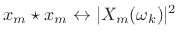
- ... projection4.17
- The coefficient of projection of a signal
onto another signal
 can be thought of as a measure of how much of
is present in
. We will consider this topic in some detail
later on.
can be thought of as a measure of how much of
is present in
. We will consider this topic in some detail
later on.
.
.
.
.
.
.
.
.
.
.
.
.
.
.
.
.
.
.
.
.
.
.
.
.
.
.
.
.
.
.
- ...vector5.1
- We'll use an underline to emphasize the vector
interpretation, but there is no difference between
and
 . For
purposes of this book, a signal is the same thing as a
vector.
. For
purposes of this book, a signal is the same thing as a
vector.
.
.
.
.
.
.
.
.
.
.
.
.
.
.
.
.
.
.
.
.
.
.
.
.
.
.
.
.
.
.
- ... hear,5.2
- Actually,
two-sample signals with variable amplitude and spacing between the
samples provide very interesting tests of pitch perception, especially
when the samples have opposite sign [57].
.
.
.
.
.
.
.
.
.
.
.
.
.
.
.
.
.
.
.
.
.
.
.
.
.
.
.
.
.
.
- ... numbers.5.3
- More generally, scalars are
often defined as members of some mathematical field--usually
the same field used for the vector elements (coordinates, signal
samples).
.
.
.
.
.
.
.
.
.
.
.
.
.
.
.
.
.
.
.
.
.
.
.
.
.
.
.
.
.
.
- ... type,5.4
- As we'll discuss in §5.7
below, vectors of the ``same type'' are typically taken to be members
of the same vector space.
.
.
.
.
.
.
.
.
.
.
.
.
.
.
.
.
.
.
.
.
.
.
.
.
.
.
.
.
.
.
- ... samples:5.5
- In this section,
denotes a signal, while in the previous sections, we used an underline
(
) to emphasize the vector interpretation of a signal. One might
worry that it is now too easy to confuse signals (vectors) and scale
factors (scalars), but this is usually not the case: signal names are
generally taken from the end of the Roman alphabet (
 ),
while scalar symbols are chosen from the beginning of the Roman
(
),
while scalar symbols are chosen from the beginning of the Roman
(
 ) and Greek (
 ) alphabets. Also, formulas involving signals are typlically
specified on the sample level, so that signals are usually indexed
(
) alphabets. Also, formulas involving signals are typlically
specified on the sample level, so that signals are usually indexed
( ) or subscripted (
 ).
).
.
.
.
.
.
.
.
.
.
.
.
.
.
.
.
.
.
.
.
.
.
.
.
.
.
.
.
.
.
.
- ... units.5.6
- The energy of a
pressure wave is the integral over time and area of the squared pressure
divided by the wave impedance the wave is traveling in. The energy of
a velocity wave is the integral over time of the squared
velocity times the wave impedance. In audio work, a signal
is
typically a list of pressure samples derived from a microphone
signal, or it might be samples of force from a piezoelectric
transducer, velocity from a magnetic guitar pickup, and so on.
In all of these cases, the total physical energy associated with the
signal is proportional to the sum of squared signal samples. Physical
connections in signal processing are explored more fully in Book III
of the Music Signal Processing Series [72], (available
online).
.
.
.
.
.
.
.
.
.
.
.
.
.
.
.
.
.
.
.
.
.
.
.
.
.
.
.
.
.
.
- ...
removed:5.7
- For reasons beyond the scope of this book, when the
sample mean
 is estimated as the average value of the same
samples used to compute the sample variance
is estimated as the average value of the same
samples used to compute the sample variance
 , the sum
should be divided by
, the sum
should be divided by  rather than
to avoid a bias
[34].
rather than
to avoid a bias
[34].
.
.
.
.
.
.
.
.
.
.
.
.
.
.
.
.
.
.
.
.
.
.
.
.
.
.
.
.
.
.
- ... vector.5.8
- You might wonder why the norm of
is
not written as
 . There would be no problem with this
since
is otherwise undefined for vectors.
However, the historically adopted notation is
instead
.
. There would be no problem with this
since
is otherwise undefined for vectors.
However, the historically adopted notation is
instead
.
.
.
.
.
.
.
.
.
.
.
.
.
.
.
.
.
.
.
.
.
.
.
.
.
.
.
.
.
.
.
- ... by5.9
- From some points of view, it is more elegant to
conjugate the first operand in the definition of the inner
product. However, for explaining the DFT, conjugating the second
operand is better. The former case arises when expressing inner
product
 as a vector operation
 , where
 denotes the
Hermitian transpose of
the vector
denotes the
Hermitian transpose of
the vector
 . Either convention works out fine, but it is best to
choose one and stick with it forever.
. Either convention works out fine, but it is best to
choose one and stick with it forever.
.
.
.
.
.
.
.
.
.
.
.
.
.
.
.
.
.
.
.
.
.
.
.
.
.
.
.
.
.
.
- ...
product:5.10
- Remember that a norm must be a real-valued
function of a signal (vector).
.
.
.
.
.
.
.
.
.
.
.
.
.
.
.
.
.
.
.
.
.
.
.
.
.
.
.
.
.
.
- ...5.11
- Note that we have dropped the underbar notation for
signals/vectors such as
 and
and
 . While this is commonly
done, it is now possible to confuse vectors and scalars. The context
should keep everything clear. Also, symbols for scalars tend to be
chosen from the beginning of the alphabet (Roman or Greek), such as
. While this is commonly
done, it is now possible to confuse vectors and scalars. The context
should keep everything clear. Also, symbols for scalars tend to be
chosen from the beginning of the alphabet (Roman or Greek), such as
 , while symbols for vectors/signals are
normally chosen from letters near the end, such as
--all
of which we have seen up to now. In later sections, the underbar
notation will continue to be used when it seems to add clarity.
, while symbols for vectors/signals are
normally chosen from letters near the end, such as
--all
of which we have seen up to now. In later sections, the underbar
notation will continue to be used when it seems to add clarity.
.
.
.
.
.
.
.
.
.
.
.
.
.
.
.
.
.
.
.
.
.
.
.
.
.
.
.
.
.
.
- ...
definition,5.12
- Note that, in this section,
denotes an entire
signal while
 denotes the
th sample of that
signal. It would be clearer to use
, but the expressions below
would become messier. In other contexts, outside of this section,
denotes the
th sample of that
signal. It would be clearer to use
, but the expressions below
would become messier. In other contexts, outside of this section,
 might instead denote the
th signal
might instead denote the
th signal
 from a set of
signals.
from a set of
signals.
.
.
.
.
.
.
.
.
.
.
.
.
.
.
.
.
.
.
.
.
.
.
.
.
.
.
.
.
.
.
- ...Noble.5.13
- An excellent collection of free downloadable course videos by Prof. Strang at MIT
is available at
http://web.mit.edu/18.06/www/Video/video-fall-99-new.html
.
.
.
.
.
.
.
.
.
.
.
.
.
.
.
.
.
.
.
.
.
.
.
.
.
.
.
.
.
.
- ...).6.1
- The Matlab code for generating this figure is given
in §I.4.1.
.
.
.
.
.
.
.
.
.
.
.
.
.
.
.
.
.
.
.
.
.
.
.
.
.
.
.
.
.
.
- ... unity.6.2
- The notations
 ,
,  , and
, and  are
common in the digital signal processing literature. Sometimes
is defined with a negative exponent, i.e.,
are
common in the digital signal processing literature. Sometimes
is defined with a negative exponent, i.e.,
 .
.
.
.
.
.
.
.
.
.
.
.
.
.
.
.
.
.
.
.
.
.
.
.
.
.
.
.
.
.
.
.
- ...
by6.3
- As introduced in §1.3, the notation
 means the whole signal
,
means the whole signal
,
 , also written as simply
.
, also written as simply
.
.
.
.
.
.
.
.
.
.
.
.
.
.
.
.
.
.
.
.
.
.
.
.
.
.
.
.
.
.
.
- ....6.4
- More
precisely,
 is a length
finite-impulse-response (FIR)
digital filter. See §8.3 for related discussion.
is a length
finite-impulse-response (FIR)
digital filter. See §8.3 for related discussion.
.
.
.
.
.
.
.
.
.
.
.
.
.
.
.
.
.
.
.
.
.
.
.
.
.
.
.
.
.
.
- ...
computed,6.5
- We call this the
aliased sinc function
to distinguish it from the sinc function
sinc
 .
.
.
.
.
.
.
.
.
.
.
.
.
.
.
.
.
.
.
.
.
.
.
.
.
.
.
.
.
.
.
.
- ...dftfilterb6.6
- The Matlab code for this figure is
given in §I.4.2.
.
.
.
.
.
.
.
.
.
.
.
.
.
.
.
.
.
.
.
.
.
.
.
.
.
.
.
.
.
.
- ....6.7
- Spectral leakage is essentially equivalent to (i.e., a
Fourier dual of) the Gibb's phenomenon for truncated Fourier
series expansions (see §B.3), which some of us studied in high
school. As more sinusoids are added to the expansion, the error
waveform increases in frequency, and decreases in signal energy, but
its peak value does not converge to zero. Instead, in the limit as
infinitely many sinusoids are added to the Fourier-series sum, the
peak error converges to an isolated point. Isolated points
have ``measure zero'' under integration, and therefore have no effect
on integrals such as the one which calculates Fourier-series
coefficients.
.
.
.
.
.
.
.
.
.
.
.
.
.
.
.
.
.
.
.
.
.
.
.
.
.
.
.
.
.
.
- ....7.1
- The notation
 denotes the
half-open interval on the real line from
denotes the
half-open interval on the real line from  to
to  .
Thus the interval includes
but not
.
.
Thus the interval includes
but not
.
.
.
.
.
.
.
.
.
.
.
.
.
.
.
.
.
.
.
.
.
.
.
.
.
.
.
.
.
.
.
- ...
spectra7.2
- A spectrum is mathematically identical to a signal, since
both are just sequences of
complex numbers. However, for clarity, we
generally use ``signal'' when the sequence index is considered a time
index, and ``spectrum'' when the index is associated with successive
frequency samples.
.
.
.
.
.
.
.
.
.
.
.
.
.
.
.
.
.
.
.
.
.
.
.
.
.
.
.
.
.
.
- ...:7.3
- The set of all integers is denoted
 .
.
.
.
.
.
.
.
.
.
.
.
.
.
.
.
.
.
.
.
.
.
.
.
.
.
.
.
.
.
.
.
- ...
convolution).7.4
- To simulate acyclic convolution using cyclic
convolution, as is appropriate for the simulation of sampled
continuous-time systems, sufficient zero padding is used so
that nonzero samples do not ``wrap around'' as a result of the
shifting of
in the definition of convolution. Zero padding is
discussed later in this
chapter (§7.2.7).
.
.
.
.
.
.
.
.
.
.
.
.
.
.
.
.
.
.
.
.
.
.
.
.
.
.
.
.
.
.
- ...7.5
- See §8.3 for an introduction to the digital-filter point
of view.
.
.
.
.
.
.
.
.
.
.
.
.
.
.
.
.
.
.
.
.
.
.
.
.
.
.
.
.
.
.
- ... exponential.7.6
- Normally, in practice, a
first-order recursive filter would be used to provide such an
exponential impulse response very efficiently in hardware or software
(see Book II [71] of this series for details). However, the impulse
response of any linear, time-invariant filter can be recorded and used
for implementation via convolution. The only catch is that recursive
filters generally have infinitely long impulse responses (true
exponential decays). Therefore, it is necessary to truncate the impulse
response when it decays enough that the remainder is negligible.
.
.
.
.
.
.
.
.
.
.
.
.
.
.
.
.
.
.
.
.
.
.
.
.
.
.
.
.
.
.
- ....7.7
- Matched filtering is briefly
discussed in §8.4.
.
.
.
.
.
.
.
.
.
.
.
.
.
.
.
.
.
.
.
.
.
.
.
.
.
.
.
.
.
.
- ...
place.7.8
- This is the also basis of the puzzle ``multiply your
age times 7 times 1443.''
.
.
.
.
.
.
.
.
.
.
.
.
.
.
.
.
.
.
.
.
.
.
.
.
.
.
.
.
.
.
- ....7.9
- The symbol ``
 ''
means ``is equivalent to''.
''
means ``is equivalent to''.
.
.
.
.
.
.
.
.
.
.
.
.
.
.
.
.
.
.
.
.
.
.
.
.
.
.
.
.
.
.
- ... domain.7.10
- Similarly, zero padding in the
frequency domain gives what we may call ``periodic interpolation'' in the
time domain which is exact in the DFT case only for periodic signals
having a time-domain period equal to the DFT length. (See §6.7.)
.
.
.
.
.
.
.
.
.
.
.
.
.
.
.
.
.
.
.
.
.
.
.
.
.
.
.
.
.
.
- ... times.7.11
- You might wonder why we need this
since all indexing in
 is defined modulo
already. The answer
is that
is defined modulo
already. The answer
is that
 formally expresses a mapping from the space
of length
signals to the space
formally expresses a mapping from the space
of length
signals to the space
 of length
  signals. The
operator could alternatively be defined
as the scaling operator
signals. The
operator could alternatively be defined
as the scaling operator
 ,
,
 , where
  is any positive integer (note the increase in signal
length from
to
is any positive integer (note the increase in signal
length from
to  samples). Such a definition would better
suggest the related continuous-time Fourier theorems regarding
time/frequency scaling (see Appendix C, especially
§C.2).
samples). Such a definition would better
suggest the related continuous-time Fourier theorems regarding
time/frequency scaling (see Appendix C, especially
§C.2).
.
.
.
.
.
.
.
.
.
.
.
.
.
.
.
.
.
.
.
.
.
.
.
.
.
.
.
.
.
.
- ....7.12
- The function
 is also considered odd,
ignoring the singularity at
is also considered odd,
ignoring the singularity at  .
.
.
.
.
.
.
.
.
.
.
.
.
.
.
.
.
.
.
.
.
.
.
.
.
.
.
.
.
.
.
.
- ... transform,7.13
- The discrete cosine transform (DCT)
used most often in applications is defined somewhat differently
(see §A.6.1), but this is one variant.
.
.
.
.
.
.
.
.
.
.
.
.
.
.
.
.
.
.
.
.
.
.
.
.
.
.
.
.
.
.
- ....7.14
- To consider
 as radians per second
instead of radians per sample, just replace
as radians per second
instead of radians per sample, just replace  by
by  so that
the delay is in seconds instead of samples, i.e.,
so that
the delay is in seconds instead of samples, i.e.,
 .
.
.
.
.
.
.
.
.
.
.
.
.
.
.
.
.
.
.
.
.
.
.
.
.
.
.
.
.
.
.
.
- ... response.7.15
- See
§8.3 and/or Book II [71] of the music signal processing
book series for an introduction to digital filters.
.
.
.
.
.
.
.
.
.
.
.
.
.
.
.
.
.
.
.
.
.
.
.
.
.
.
.
.
.
.
- ... Transform7.16
- An FFT is just a fast implementation of
the DFT. See Appendix A for details and pointers.
.
.
.
.
.
.
.
.
.
.
.
.
.
.
.
.
.
.
.
.
.
.
.
.
.
.
.
.
.
.
- ... FFT.7.17
- These results were
obtained using the program Octave, version 2.9.9, running on
a Linux PC with a 2.8GHz Pentium CPU, and Matlab, version
5.2, running on a Windows PC with an 800MHz Athlon CPU.
.
.
.
.
.
.
.
.
.
.
.
.
.
.
.
.
.
.
.
.
.
.
.
.
.
.
.
.
.
.
- ...table:ffttable.7.18
- These results were obtained using
Matlab v5.2 running on a Windows PC with an 800MHz
Athlon CPU.
.
.
.
.
.
.
.
.
.
.
.
.
.
.
.
.
.
.
.
.
.
.
.
.
.
.
.
.
.
.
- ...dual7.19
- The dual of a Fourier operation
is obtained by interchanging time and frequency.
.
.
.
.
.
.
.
.
.
.
.
.
.
.
.
.
.
.
.
.
.
.
.
.
.
.
.
.
.
.
- ... time.7.20
- Signal processing with a physical
interpretation is addressed in Book III [72] of the music
signal processing series.
.
.
.
.
.
.
.
.
.
.
.
.
.
.
.
.
.
.
.
.
.
.
.
.
.
.
.
.
.
.
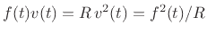
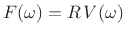
- ....7.21
- You might be
concerned about what it means when
 has an
imaginary part. This happens when the force
has an
imaginary part. This happens when the force  drives a
so-called ``reactive'' load such as a mass or spring. For the
details, see Book III [72] or any text on classical network
theory or circuit theory. When the driving force
works against
a real resistance
drives a
so-called ``reactive'' load such as a mass or spring. For the
details, see Book III [72] or any text on classical network
theory or circuit theory. When the driving force
works against
a real resistance  , then
 (see §F.3), so
that the power is
(see §F.3), so
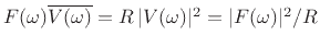
that the power is
 , and in the frequency
domain,
, and in the frequency
domain,
 so that the spectral power is
proportional to
so that the spectral power is
proportional to
 . Thus,
in the case of a real driving-point impedance
. Thus,
in the case of a real driving-point impedance  , the spectral power
is always real and nonnegative.
, the spectral power
is always real and nonnegative.
.
.
.
.
.
.
.
.
.
.
.
.
.
.
.
.
.
.
.
.
.
.
.
.
.
.
.
.
.
.
- ... frequency7.22
- The
folding frequency is defined as half the sampling rate
 .
It may also be called the Nyquist limit. The Nyquist
rate, on the other hand, means the sampling rate, not half
the sampling rate.
.
It may also be called the Nyquist limit. The Nyquist
rate, on the other hand, means the sampling rate, not half
the sampling rate.
.
.
.
.
.
.
.
.
.
.
.
.
.
.
.
.
.
.
.
.
.
.
.
.
.
.
.
.
.
.
- ... FIR7.23
- FIR stands for ``Finite
Impulse Response.'' Digital filtering concepts and terminology are
introduced in §8.3 and more completely in Book II [71]
of the music signal processing series.
.
.
.
.
.
.
.
.
.
.
.
.
.
.
.
.
.
.
.
.
.
.
.
.
.
.
.
.
.
.
- ...CooleyAndTukey65.8.1
- While a length
DFT requires
approximately
 arithmetic operations, a Cooley-Tukey FFT requires
closer to
arithmetic operations, a Cooley-Tukey FFT requires
closer to
 operations when
  is a power of 2, where
 denotes the log-base-2 of
. Appendix A provides an
introduction to Cooley-Tukey FFT algorithms in §A.1.
denotes the log-base-2 of
. Appendix A provides an
introduction to Cooley-Tukey FFT algorithms in §A.1.
.
.
.
.
.
.
.
.
.
.
.
.
.
.
.
.
.
.
.
.
.
.
.
.
.
.
.
.
.
.
- ....8.2
- Say ``doc fft'' in Matlab for an overview of
how a specific FFT algorithm is chosen.
.
.
.
.
.
.
.
.
.
.
.
.
.
.
.
.
.
.
.
.
.
.
.
.
.
.
.
.
.
.
- ...SASP8.3
- http://ccrma.stanford.edu/~jos/sasp/Classic_Blackman.html
.
.
.
.
.
.
.
.
.
.
.
.
.
.
.
.
.
.
.
.
.
.
.
.
.
.
.
.
.
.
- ... Octave8.4
- http://www.octave.org/
.
.
.
.
.
.
.
.
.
.
.
.
.
.
.
.
.
.
.
.
.
.
.
.
.
.
.
.
.
.
- ... Toolbox,8.5
- http://www.mathworks.com/access/helpdesk/help/toolbox/signal/signal.shtml
.
.
.
.
.
.
.
.
.
.
.
.
.
.
.
.
.
.
.
.
.
.
.
.
.
.
.
.
.
.
- ...
phoneme,8.6
- A phoneme is a single elementary sound in
speech, such as a single vowel sound like the `a' in ``bat'' or the
`s' in ``sit''.
.
.
.
.
.
.
.
.
.
.
.
.
.
.
.
.
.
.
.
.
.
.
.
.
.
.
.
.
.
.
- ...
system8.7
- Linearity and time invariance are introduced in
the second book of this series [71].
.
.
.
.
.
.
.
.
.
.
.
.
.
.
.
.
.
.
.
.
.
.
.
.
.
.
.
.
.
.
- ...estimator8.8
- In signal processing, a ``hat'' often denotes an estimated quantity.
Thus,
 is an estimate of
  .
.
.
.
.
.
.
.
.
.
.
.
.
.
.
.
.
.
.
.
.
.
.
.
.
.
.
.
.
.
.
.
- ...
value8.9
- For present purposes, the expected value
may be found by averaging an infinite number of
cross-correlations
 computed using different segments of
and
. Both
and
must be infinitely long, of course, and
all stationary processes
are infinitely long. Otherwise, their statistics could not be
time invariant.
computed using different segments of
and
. Both
and
must be infinitely long, of course, and
all stationary processes
are infinitely long. Otherwise, their statistics could not be
time invariant.
.
.
.
.
.
.
.
.
.
.
.
.
.
.
.
.
.
.
.
.
.
.
.
.
.
.
.
.
.
.
- ... PSD:8.10
- To clarify, we are using the word ``sample'' with
two different meanings. In addition to the usual meaning wherein a
continuous time or frequency axis is made discrete, a statistical
``sample'' refers to a set of observations from some presumed random
process. Estimated statistics based on such a statistical sample are
then called ``sample statistics'', such as the sample mean, sample
variance, and so on.
.
.
.
.
.
.
.
.
.
.
.
.
.
.
.
.
.
.
.
.
.
.
.
.
.
.
.
.
.
.
- ....8.11
- See
Eq.(7.1) for a definition of
 .
.
.
.
.
.
.
.
.
.
.
.
.
.
.
.
.
.
.
.
.
.
.
.
.
.
.
.
.
.
.
.
- ...https://ccrma.stanford.edu/ jos/mdft/mdft-python.html#FIR-System-Identification8.12
- https://ccrma.stanford.edu/~jos/mdft/mdft-python.html#FIR-System-Identification
.
.
.
.
.
.
.
.
.
.
.
.
.
.
.
.
.
.
.
.
.
.
.
.
.
.
.
.
.
.
- ....8.13
- Since phase information is discarded
(
 ),
the zero-padding can go before or after
),
the zero-padding can go before or after  ,
or both, without affecting the results.
,
or both, without affecting the results.
.
.
.
.
.
.
.
.
.
.
.
.
.
.
.
.
.
.
.
.
.
.
.
.
.
.
.
.
.
.
- ... kernel;8.14
- By the convolution theorem dual, windowing
in the time domain is convolution (smoothing) in the frequency domain
(§7.4.6). Since a triangle is the convolution of a
rectangle with itself, its transform is
sinc
 in the
continuous-time case (cf. Appendix D). In the discrete-time
case, it is proportional to
in the
continuous-time case (cf. Appendix D). In the discrete-time
case, it is proportional to
 sinc
sinc .
.
.
.
.
.
.
.
.
.
.
.
.
.
.
.
.
.
.
.
.
.
.
.
.
.
.
.
.
.
.
.
- ...https://ccrma.stanford.edu/ jos/mdft/mdft-python.html#Coherence-Function-in-Matlab8.15
- https://ccrma.stanford.edu/~jos/mdft/mdft-python.html#Coherence-Function-in-Matlab
.
.
.
.
.
.
.
.
.
.
.
.
.
.
.
.
.
.
.
.
.
.
.
.
.
.
.
.
.
.
- ...
compositeA.1
- In this context, ``highly composite'' means ``a
product of many prime factors.'' For example, the number
 is highly composite since it is a power of 2. The
number
is highly composite since it is a power of 2. The
number
 is also composite, but it
requires prime factors other than 2. Prime numbers
is also composite, but it
requires prime factors other than 2. Prime numbers
 are not composite at all.
.
.
.
.
.
.
.
.
.
.
.
.
.
.
.
.
.
.
.
.
.
.
.
.
.
.
.
.
.
.
- ...A.2
- See
http://en.wikipedia.org/wiki/Cooley-Tukey_FFT_algorithm.
.
.
.
.
.
.
.
.
.
.
.
.
.
.
.
.
.
.
.
.
.
.
.
.
.
.
.
.
.
.
- ...DuhamelAndVetterli90.A.3
- http://en.wikipedia.org/wiki/Split_radix
.
.
.
.
.
.
.
.
.
.
.
.
.
.
.
.
.
.
.
.
.
.
.
.
.
.
.
.
.
.
- ...Good58,Thomas63,KolbaAndParks77,McClellanAndRader79,BurrusAndParks85,WikiPFA.A.4
- See
http://en.wikipedia.org/wiki/Prime-factor_FFT_algorithm
for an
introduction.
.
.
.
.
.
.
.
.
.
.
.
.
.
.
.
.
.
.
.
.
.
.
.
.
.
.
.
.
.
.
- ...A.5
- http://en.wikipedia.org/wiki/Prime-factor_FFT_algorithm#Re-indexing
.
.
.
.
.
.
.
.
.
.
.
.
.
.
.
.
.
.
.
.
.
.
.
.
.
.
.
.
.
.
- ...GoldAndRader69.A.6
- See
http://en.wikipedia.org/wiki/Bluestein's_FFT_algorithm
for another
derivation and description of Bluestein's FFT algorithm.
.
.
.
.
.
.
.
.
.
.
.
.
.
.
.
.
.
.
.
.
.
.
.
.
.
.
.
.
.
.
- ...
unity,A.7
- Note that
 is the complex-conjugate of
used
in §A.1.1 above.
is the complex-conjugate of
used
in §A.1.1 above.
.
.
.
.
.
.
.
.
.
.
.
.
.
.
.
.
.
.
.
.
.
.
.
.
.
.
.
.
.
.
- ...
length.A.8
- Obtaining an exact integer number of samples per
period can be arranged using pitch detection and
resampling of the periodic signal. A time-varying pitch
requires time-varying resampling [75]--see
Appendix D. However, when a signal is resampled for this purpose,
one can generally choose a power of 2 for the number of samples per
period.
.
.
.
.
.
.
.
.
.
.
.
.
.
.
.
.
.
.
.
.
.
.
.
.
.
.
.
.
.
.
- ... gain.A.9
- This result is well known in the field of
image processing. The DCT performs almost as well as the optimal
Karhunen-Loève Transform (KLT) when analyzing certain Gaussian
stochastic processes as the transform size goes to infinity. (In the
KLT, the basis functions are taken to be the eigenvectors of the
autocorrelation matrix of the input signal block. As a result, the
transform coefficients are decorrelated in the KLT, leading to
maximum energy concentration and optimal coding gain.) However, the
DFT provides a similar degree of optimality for large block sizes
.
For practical spectral analysis and processing of audio signals, there
is typically no reason to prefer the DCT over the DFT.
.
.
.
.
.
.
.
.
.
.
.
.
.
.
.
.
.
.
.
.
.
.
.
.
.
.
.
.
.
.
- ...
DCT-II)A.10
- For a discussion of eight or so DCT variations,
see the Wikipedia page:
http://en.wikipedia.org/wiki/Discrete_cosine_transform
.
.
.
.
.
.
.
.
.
.
.
.
.
.
.
.
.
.
.
.
.
.
.
.
.
.
.
.
.
.
- ...FFTWPaper.A.11
- For a list of FFT implementations benchmarked against
FFTW, see http://www.fftw.org/benchfft/ffts.html
.
.
.
.
.
.
.
.
.
.
.
.
.
.
.
.
.
.
.
.
.
.
.
.
.
.
.
.
.
.
- ... variable,B.1
- We
define the DTFT using normalized radian frequency
 .
.
.
.
.
.
.
.
.
.
.
.
.
.
.
.
.
.
.
.
.
.
.
.
.
.
.
.
.
.
.
.
- ...
seconds,B.2
- A signal
is said to be periodic with
period
 if
if
 for all
 .
.
.
.
.
.
.
.
.
.
.
.
.
.
.
.
.
.
.
.
.
.
.
.
.
.
.
.
.
.
.
.
- ... isB.3
- To obtain precisely this
result, it is necessary to define
 via a limiting pulse
converging to time 0 from the right of time 0, as we have done
in Eq.(B.3).
via a limiting pulse
converging to time 0 from the right of time 0, as we have done
in Eq.(B.3).
.
.
.
.
.
.
.
.
.
.
.
.
.
.
.
.
.
.
.
.
.
.
.
.
.
.
.
.
.
.
- ... principle|textbf.C.1
- The Heisenberg uncertainty principle in quantum physics
applies to any dual properties of a particle. For example, the
position and velocity of an electron are oft-cited as such duals. An
electron is described, in quantum mechanics, by a probability wave
packet. Therefore, the position of an electron in space can be
defined as the midpoint of the amplitude envelope of its wave
function; its velocity, on the other hand, is determined by the
frequency of the wave packet. To accurately measure the
frequency, the packet must be very long in space, to provide many
cycles of oscillation under the envelope. But this means the location
in space is relatively uncertain. In more precise mathematical terms,
the probability wave function for velocity is proportional to the
spatial Fourier transform of the probability wave for position. I.e.,
they are exact Fourier duals. The Heisenberg Uncertainty Principle is
therefore a Fourier property of fundamental particles described by
waves [20]. This of course includes all matter and energy in the
Universe.
.
.
.
.
.
.
.
.
.
.
.
.
.
.
.
.
.
.
.
.
.
.
.
.
.
.
.
.
.
.
- ... filter.C.2
- An allpass filter has unity gain and
arbitrary delay at each frequency.
.
.
.
.
.
.
.
.
.
.
.
.
.
.
.
.
.
.
.
.
.
.
.
.
.
.
.
.
.
.
- ... public.D.1
- http://cnx.org/content/m0050/latest/
.
.
.
.
.
.
.
.
.
.
.
.
.
.
.
.
.
.
.
.
.
.
.
.
.
.
.
.
.
.
- ...
positionD.2
- More typically, each sample represents the
instantaneous velocity of the speaker. Here's why: Most
microphones are transducers from acoustic pressure to
electrical voltage, and analog-to-digital converters (ADCs)
produce numerical samples which are proportional to voltage. Thus,
digital samples are normally proportional to acoustic pressure
deviation (force per unit area on the microphone, with ambient air
pressure subtracted out). When digital samples are converted to
analog form by digital-to-analog conversion (DAC), each sample is
converted to an electrical voltage which then drives a loudspeaker (in
audio applications). Typical loudspeakers use a ``voice-coil'' to
convert applied voltage to electromotive force on the speaker which
applies pressure on the air via the speaker cone. Since the acoustic
impedance of air is a real number, wave pressure is directly
proportional wave velocity. Since the speaker must move in
contact with the air during wave generation, we may conclude that
digital signal samples correspond most closely to the velocity
of the speaker, not its position. The situation is further
complicated somewhat by the fact that typical speakers do not
themselves have a real driving-point impedance.
However, for an ``ideal'' microphone and speaker, we should get
samples proportional to speaker velocity and hence to air pressure.
Well below resonance, the real part of the radiation impedance
of the pushed air
should dominate, as long as the excursion does not exceed the linear
interval of cone displacement.
.
.
.
.
.
.
.
.
.
.
.
.
.
.
.
.
.
.
.
.
.
.
.
.
.
.
.
.
.
.
- ....D.3
- Mathematically,
 can be allowed to be nonzero over points
 provided that the set of all such points have measure zero in
the sense of Lebesgue integration. However, such distinctions do not
arise for practical signals which are always finite in extent and
which therefore have continuous Fourier transforms. This is why we
specialize the sampling theorem to the case of continuous-spectrum
signals.
provided that the set of all such points have measure zero in
the sense of Lebesgue integration. However, such distinctions do not
arise for practical signals which are always finite in extent and
which therefore have continuous Fourier transforms. This is why we
specialize the sampling theorem to the case of continuous-spectrum
signals.
.
.
.
.
.
.
.
.
.
.
.
.
.
.
.
.
.
.
.
.
.
.
.
.
.
.
.
.
.
.
- ... pulse,E.1
- Thanks to Miller
Puckette for suggesting this example.
.
.
.
.
.
.
.
.
.
.
.
.
.
.
.
.
.
.
.
.
.
.
.
.
.
.
.
.
.
.
- ... energy).E.2
- One joke along these lines, due, I'm
told, to Professor Bracewell at Stanford, is that ``since the
telephone is bandlimited to 3kHz, and since bandlimited signals cannot
be time limited, it follows that one cannot hang up the telephone''.
.
.
.
.
.
.
.
.
.
.
.
.
.
.
.
.
.
.
.
.
.
.
.
.
.
.
.
.
.
.
- ... belF.1
- The ``bel'' is named after Alexander
Graham Bell, the inventor of the telephone.
.
.
.
.
.
.
.
.
.
.
.
.
.
.
.
.
.
.
.
.
.
.
.
.
.
.
.
.
.
.
- ... intensity,F.2
-
Intensity is
physically power per unit area. Bels may also be defined in
terms of energy, or power which is energy per unit time.
Since sound is always measured over some
area by a microphone diaphragm, its physical power is conventionally
normalized by area, giving intensity. Similarly, the force applied
by sound to a microphone diaphragm is normalized by area to give
pressure (force per unit area).
.
.
.
.
.
.
.
.
.
.
.
.
.
.
.
.
.
.
.
.
.
.
.
.
.
.
.
.
.
.
- ... ScaleF.3
- This section was added in the third printing of this
book (September 2013).
.
.
.
.
.
.
.
.
.
.
.
.
.
.
.
.
.
.
.
.
.
.
.
.
.
.
.
.
.
.
- ... ScaleF.4
- This section was added in the third printing of this
book (September 2013).
.
.
.
.
.
.
.
.
.
.
.
.
.
.
.
.
.
.
.
.
.
.
.
.
.
.
.
.
.
.
- ...LobdellAndAllen07.F.5
- For other software implementations, see,e.g.,
http://kokkinizita.linuxaudio.org/linuxaudio/,
https://github.com/x42/meters.lv2
.
.
.
.
.
.
.
.
.
.
.
.
.
.
.
.
.
.
.
.
.
.
.
.
.
.
.
.
.
.
- ... isF.6
- The bar was originally defined as one ``atmosphere'' (atmospheric pressure at sea level),
but now a microbar is defined to be exactly one
dyne
 cm
,
where a dyne is the amount of force required to accelerate a gram by one centimeter
per second squared.
cm
,
where a dyne is the amount of force required to accelerate a gram by one centimeter
per second squared.
.
.
.
.
.
.
.
.
.
.
.
.
.
.
.
.
.
.
.
.
.
.
.
.
.
.
.
.
.
.
- ....F.7
- Standard International (SI) units were formerly
called MKS units (meters, kilograms, and seconds).
.
.
.
.
.
.
.
.
.
.
.
.
.
.
.
.
.
.
.
.
.
.
.
.
.
.
.
.
.
.
- ...
phons.F.8
- See
http://en.wikipedia.org/wiki/A-weighting
for more information, including a plot of the A weighting curve (as
well as B, C, and D weightings which can be used for louder listening
levels) and pointers to relevant standards.
.
.
.
.
.
.
.
.
.
.
.
.
.
.
.
.
.
.
.
.
.
.
.
.
.
.
.
.
.
.
- ... byF.9
- ibid.
.
.
.
.
.
.
.
.
.
.
.
.
.
.
.
.
.
.
.
.
.
.
.
.
.
.
.
.
.
.
- ... weighting|textbfF.10
- http://en.wikipedia.org/wiki/ITU-R_468_noise_weighting
.
.
.
.
.
.
.
.
.
.
.
.
.
.
.
.
.
.
.
.
.
.
.
.
.
.
.
.
.
.
- ...
distortion'').F.11
- Companders (compressor-expanders) essentially
``turn down'' the signal gain when it is ``loud'' and ``turn up'' the
gain when it is ``quiet''. As long as the input-output curve is
monotonic (such as a log characteristic), the dynamic-range
compression can be undone (expanded).
.
.
.
.
.
.
.
.
.
.
.
.
.
.
.
.
.
.
.
.
.
.
.
.
.
.
.
.
.
.
- ... 0.G.1
- Computers use bits, as opposed to the more
familiar decimal digits, because they are more convenient to implement
in digital hardware. For example, the decimal numbers 0, 1, 2,
3, 4, 5 become, in binary format, 0, 1, 10, 11, 100, 101. Each
bit position in binary notation corresponds to a power of 2,
e.g.,
 ; while each
digit position in decimal notation corresponds to a power of
10, e.g.,
; while each
digit position in decimal notation corresponds to a power of
10, e.g.,
 . The term
``digit'' comes from the same word meaning ``finger.'' Since
we have ten fingers (digits), the term ``digit'' technically should be
associated only with decimal notation, but in practice it is used for
others as well. Other popular number systems in computers include
octal which is base 8 (rarely seen any more, but still
specifiable in any C/C++ program by using a leading zero, e.g.,
. The term
``digit'' comes from the same word meaning ``finger.'' Since
we have ten fingers (digits), the term ``digit'' technically should be
associated only with decimal notation, but in practice it is used for
others as well. Other popular number systems in computers include
octal which is base 8 (rarely seen any more, but still
specifiable in any C/C++ program by using a leading zero, e.g.,
 decimal = 111,101,101
binary), and hexadecimal (or simply ``hex'') which is
base 16 and which employs the letters A through F to yield 16 digits
(specifiable in C/C++ by starting the number with ``0x'', e.g., 0x1ED
=
decimal = 111,101,101
binary), and hexadecimal (or simply ``hex'') which is
base 16 and which employs the letters A through F to yield 16 digits
(specifiable in C/C++ by starting the number with ``0x'', e.g., 0x1ED
=
 decimal =
1,1110,1101 binary). Note, however, that the representation within
the computer is still always binary; octal and hex are simply
convenient groupings of bits into sets of three bits (octal)
or four bits (hex).
decimal =
1,1110,1101 binary). Note, however, that the representation within
the computer is still always binary; octal and hex are simply
convenient groupings of bits into sets of three bits (octal)
or four bits (hex).
.
.
.
.
.
.
.
.
.
.
.
.
.
.
.
.
.
.
.
.
.
.
.
.
.
.
.
.
.
.
- ... processors.G.2
- This information is subject to change
without notice. Check your local compiler documentation.
.
.
.
.
.
.
.
.
.
.
.
.
.
.
.
.
.
.
.
.
.
.
.
.
.
.
.
.
.
.
- ... feedbackG.3
- Normally, quantization error
is computed as
 , where
is the signal being
quantized, and
, where
is the signal being
quantized, and
![$ {\hat x}(n) = Q[x(n)]$](img1998.png) is the quantized value, obtained by
rounding to the nearest representable amplitude. Filtered error
feedback uses instead the formula
is the quantized value, obtained by
rounding to the nearest representable amplitude. Filtered error
feedback uses instead the formula
![$ {\hat x}(n) = Q[x(n)+{\cal L}\{e(n-1)\}]$](img1999.png) ,
where
,
where
 denotes a filtering operation which ``shapes'' the
quantization noise spectrum. An excellent article on the use of
round-off error feedback in audio digital filters is
[18].
denotes a filtering operation which ``shapes'' the
quantization noise spectrum. An excellent article on the use of
round-off error feedback in audio digital filters is
[18].
.
.
.
.
.
.
.
.
.
.
.
.
.
.
.
.
.
.
.
.
.
.
.
.
.
.
.
.
.
.
- ... Bytes?G.4
- This subsection can be skipped if you are using only modern laptops and desktops.
.
.
.
.
.
.
.
.
.
.
.
.
.
.
.
.
.
.
.
.
.
.
.
.
.
.
.
.
.
.
- ... Bytes?G.5
- This subsection can be skipped if you are using only modern laptops and desktops.
.
.
.
.
.
.
.
.
.
.
.
.
.
.
.
.
.
.
.
.
.
.
.
.
.
.
.
.
.
.
- ... most-significant).G.6
- Remember that byte
addresses in a big endian word start at the big end of the word, while
in a little endian architecture, they start at the little end of the
word.
.
.
.
.
.
.
.
.
.
.
.
.
.
.
.
.
.
.
.
.
.
.
.
.
.
.
.
.
.
.
- ...
``endianness'':G.7
- Thanks to Bill Schottstaedt for help with this table.
.
.
.
.
.
.
.
.
.
.
.
.
.
.
.
.
.
.
.
.
.
.
.
.
.
.
.
.
.
.
- ...,G.8
- The notation
denotes a half-open interval which includes
but not
.
.
.
.
.
.
.
.
.
.
.
.
.
.
.
.
.
.
.
.
.
.
.
.
.
.
.
.
.
.
.
- ....G.9
- Another term commonly heard for ``significand''
is ``mantissa.'' However, this use of the term ``mantissa'' is not the same
as its previous definition as the fractional part of a logarithm. We will
therefore use only the term ``significand'' to avoid confusion.
.
.
.
.
.
.
.
.
.
.
.
.
.
.
.
.
.
.
.
.
.
.
.
.
.
.
.
.
.
.
- ... bias.G.10
- By choosing
the bias equal to half the numerical dynamic range of
 (thus effectively
inverting the sign bit of the exponent), it becomes easier to compare two
floating-point numbers in hardware: the entire floating-point word can be
treated by the hardware as one giant integer for numerical comparison
purposes. This works because negative exponents correspond to
floating-point numbers less than 1 in magnitude, while positive exponents
correspond to floating-point numbers greater than 1 in magnitude.
(thus effectively
inverting the sign bit of the exponent), it becomes easier to compare two
floating-point numbers in hardware: the entire floating-point word can be
treated by the hardware as one giant integer for numerical comparison
purposes. This works because negative exponents correspond to
floating-point numbers less than 1 in magnitude, while positive exponents
correspond to floating-point numbers greater than 1 in magnitude.
.
.
.
.
.
.
.
.
.
.
.
.
.
.
.
.
.
.
.
.
.
.
.
.
.
.
.
.
.
.
- ...CODEC|textbfCODECsG.11
- CODEC is an acronym for
``COder/DECoder''.
.
.
.
.
.
.
.
.
.
.
.
.
.
.
.
.
.
.
.
.
.
.
.
.
.
.
.
.
.
.
- ... processing.G.12
- The
first by Gray and Davisson is available free online. The second by
Papoulis is a classic textbook. The two volumes by Kay provide
perhaps the most comprehensive coverage of the field. The volumes by
Sharf and Kailath represent material used for many years in the
authors' respective graduate level courses in statistical signal
processing. All of the cited authors are well known researchers and
professors in the field. It should also perhaps be noted that Book IV
[73] in the music signal processing book series (of which this
is Book I) contains a fair amount of introductory material in this area.
.
.
.
.
.
.
.
.
.
.
.
.
.
.
.
.
.
.
.
.
.
.
.
.
.
.
.
.
.
.
- ...PapoulisRV:G.13
- http://en.wikipedia.org/wiki/Probability_density_function
.
.
.
.
.
.
.
.
.
.
.
.
.
.
.
.
.
.
.
.
.
.
.
.
.
.
.
.
.
.
- ... elementH.1
- We are now using
as an
integer counter, not as
. This is standard notational
practice.
.
.
.
.
.
.
.
.
.
.
.
.
.
.
.
.
.
.
.
.
.
.
.
.
.
.
.
.
.
.
- ...
argument.H.2
- Alternatively, it can be extended to the complex case by
writing
![$ \mathbf{A}^{\ast }\mathbf{B}\isdef [\ldots<b_j,a^{\ast }_i>\ldots]$](img2087.png) , so that
, so that
 includes a conjugation of the elements of
 . This
difficulty arises from the fact that matrix multiplication is really
defined without consideration of conjugation or transposition at all,
making it unwieldy to express in terms of inner products in the complex
case, even though that is perhaps the most fundamental interpretation
of a matrix multiply.
. This
difficulty arises from the fact that matrix multiplication is really
defined without consideration of conjugation or transposition at all,
making it unwieldy to express in terms of inner products in the complex
case, even though that is perhaps the most fundamental interpretation
of a matrix multiply.
.
.
.
.
.
.
.
.
.
.
.
.
.
.
.
.
.
.
.
.
.
.
.
.
.
.
.
.
.
.
- ... columns.I.1
- For consistency with sum and other
functions, it would be better if
length() returned the number of elements along dimension
1, with the special case of using dimension 2 (``along rows'') for
row-vectors. However, compatibility with early Matlab dictates
the convention used.
.
.
.
.
.
.
.
.
.
.
.
.
.
.
.
.
.
.
.
.
.
.
.
.
.
.
.
.
.
.
- ... matrix|textbf.I.2
- Going back into ``math mode'', let's show that the
 projection matrix
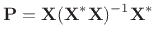 |
(I.1) |
yields orthogonal projection onto the column-space of
 (when
the
(when
the  matrix
 is invertible, and here
 denotes the Hermitian (conjugating) transpose of
). That is, if
denotes the Hermitian (conjugating) transpose of
). That is, if
 is the
projection of
onto
, we must have, by definition of
orthogonal projection (§5.9.9), that
is the
projection of
onto
, we must have, by definition of
orthogonal projection (§5.9.9), that  lies in the
column-space of
, and that
lies in the
column-space of
, and that
 , or
, or
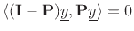 for any
 .
We may say that
.
We may say that
 projects onto the
orthogonal complement of the column-space of
.
projects onto the
orthogonal complement of the column-space of
.
That
is a linear combination of the columns of
is
immediate because
is the leftmost term of the definition of
 in Eq.(I.1). To show orthogonality of the ``projection
error'', i.e., that
for all
, note that in matrix notation we must show
in Eq.(I.1). To show orthogonality of the ``projection
error'', i.e., that
for all
, note that in matrix notation we must show
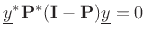 for all
 , which
requires
, which
requires
 , or
, or
 . Since
 , it is Hermitian symmetric, so
that the orthogonal projection requirement becomes
, it is Hermitian symmetric, so
that the orthogonal projection requirement becomes
 , which is easily verified for
as
defined in Eq.(I.1).
, which is easily verified for
as
defined in Eq.(I.1).
The general property
 defines an idempotent
square matrix
. Intuitively, it makes sense that a
projection should be idempotent, because once a vector is projected
onto a particular subspace, projecting again should do nothing. All
idempotent matrices are projection matrices, and vice versa. However,
only Hermitian (symmetric) idempotent matrices correspond to orthogonal
projection [48].
defines an idempotent
square matrix
. Intuitively, it makes sense that a
projection should be idempotent, because once a vector is projected
onto a particular subspace, projecting again should do nothing. All
idempotent matrices are projection matrices, and vice versa. However,
only Hermitian (symmetric) idempotent matrices correspond to orthogonal
projection [48].
.
.
.
.
.
.
.
.
.
.
.
.
.
.
.
.
.
.
.
.
.
.
.
.
.
.
.
.
.
.