Next: Numerical Phase Velocity and
Up: Finite Difference Interpretation
Previous: Finite Difference Interpretation
MDWD Networks as Multi-step Schemes
Recall that the discretization step discussed in §3.5.3 consisted of the application of a spectral transformation of the form
where  is the frequency domain transform variable corresponding to any MD-causal coordinate
  , and
, and
 is the frequency domain unit shift in the same direction.
For spatially inhomogeneous problems, this spectral mapping is equivalent to the application of the trapezoid rule in direction . We can thus write, using operator notation,
 |
(3.69) |
where
 is a shift operator defined by
when applied to any continuous function
 . Consider again the lossless (1+1)D transmission line equations
 |
(3.70a) |
which can be written as
 |
(3.71a) |
under the application of coordinate transformation (3.19) and using scaled variables  and
and
 , as well as the scaled time variable
 . Under the substitution of (3.73), for
  , and using the generalized trapezoid rule in time, defined by
where
 is a shift in the scaled time direction
  of duration
  , we get
to second order in  . This can be rewritten as
 |
(3.72a) |
where we have used
 ,
,
 , the fact that
 , and also the definitions of the port resistances of the MDWD network of Figure 3.14(b), given in (3.64)
 .
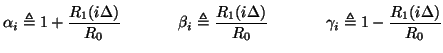
Upon replacing the quantities
.
Upon replacing the quantities  and
and  by their respective grid functions
 and
and
 , which take on values for
  and
and  integer, (3.77a) and (3.77b) define recursions on a regular grid, of spacing . (3.77a) can be written as
 |
 |
 |
(3.73) |
| |
 |
 |
(3.74) |
| |
|
 |
(3.75) |
| |
|
 |
(3.76) |
| |
|
 |
(3.77) |
with
 |
(3.78) |
The recursion corresponding to (3.77b) is very similar, under the interchange of  and
and  . Note that if
  and
and  are constants, and if the difference scheme is operating at the CFL bound (so that
 , then (3.78) can be simplified to
 |
(3.79) |
which is a simple centered difference approximation to (3.74a) and which we will see again in the waveguide mesh context in §4.3.2. Unlike the case of the mesh however, away from the passivity bound we have a multi-step scheme [176] which involves three steps of ``look-back'' in order to update a grid variable at a particular location. The introduction of wave variables, then, can be considered to be a means of expanding the state of the system so that using the new state, the recursion (now in the form of the MDWDF of Figure 3.14) requires access only to wave quantities at the time step immediately preceding the current one.
In order to generate a scheme which operates on alternating interleaved grids (called offset sampling in [61]), it is possible to use a doubled time step of
 in order to implement the generalized trapezoid rule applied to the time derivatives in (3.75a) and (3.75b), i.e.,
in which case we get, as an approximation to (3.74a),
where  and
and  are defined as per (3.79), but where
  is now equal to
 . This form also reduces to simple centered differences when and are constant, and when we are operating at the CFL bound.
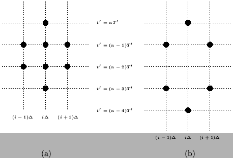
The computational stencils corresponding to the two different schemes are shown in Figure 3.20; the top black dot in either picture represents the location of the grid variable currently being updated (either or ), and the other dots cover the discrete region of influence of the difference scheme. Notice in particular that each scheme has a width of only three grid points, corresponding to nearest-neighbor-only updating. Also, because these are multi-step methods, one might expect that we will have to take special care when initializing the scheme; we discuss this issue in §3.10. For the offset scheme of Figure 3.20(b), the stencil can be shifted one step to the left or right without any overlapping; thus such a scheme can subdivided into two mutually exclusive subschemes (operating only for  always even or always odd), one of which may be dropped from the calculating scheme entirely. This behavior appears in many of the difference schemes which we will come across subsequently; we will pay particular attention to such schemes during a spectral analysis of finite difference schemes in Appendix A.
Figure 3.20:
Computational stencils of the equivalent multi-step schemes of MDWDFs for the (1+1)D transmission line equations-- (a) scheme (3.78) and (b) ``offset'' scheme (3.81).
 |
One of the interesting features of the MDKC representation of a set of PDEs is that the same circuit can give rise to an entire family of MDWD networks, or, in other words, of difference methods, all of which are consistent with the original set of PDEs. In the case of the MDKC for the transmission line equations derived previously, although we have defined the directions of the various inductors (along which we will be integrating), at the circuit stage we have not as yet specified any spectral mapping which will determine the type of differencing to be applied. Any passivity-preserving mapping which is correct in the low frequency limit will give rise to a passive, consistent MDWD algorithm. We will examine the important implications of a more exotic type of mapping in §4.10, but it is also interesting to note that we can apply the trapezoid rule using different step sizes for all the reactive elements. The constraint on our choices of these step sizes is that all shifting operations refer, ultimately, to another grid point (for computability).
Finally, we note that in general, the determination of stability for a multi-step scheme can be quite difficult; even in the constant coefficient case, it will in general be necessary to perform Von Neumann analysis [176] (see Appendix A for such an analysis applied to difference schemes for the wave equation in (2+1)D and (3+1)D), which can be quite formidable. Here, however, we are ensured stability through the passivity condition on the network.
Next: Numerical Phase Velocity and
Up: Finite Difference Interpretation
Previous: Finite Difference Interpretation
Stefan Bilbao
2002-01-22