Initial Conditions

Numerical simulations for time-dependent systems of PDEs must necessarily be initialized; while this is a relatively straightforward matter for WDF-based integration schemes, it has only been addressed in passing [106] in the literature.

We will examine here the initialization of the MDWD network for the source-free transmission line system (3.56) with $e=h=0$. This system requires initial distributions for both the current and voltage, which we will call $i_{0}(x)$ and $u_{0}(x)$, respectively. For the initialization of the MDWD network for this system (shown in Figure 3.22), we will also need their spatial derivatives (assuming they exist), which we will write as $i_{0}'(x)$ and $u_{0}'(x)$. We note that in the approach considered in [106], spatial derivative information has not been taken into account.

Figure 3.22: MDWD network for the source-free (1+1)D transmission line equations.

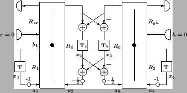For the MDWD network of Figure 3.22, we must initialize all the wave variables incident upon the scattering junctions, written as $a_{j}$, $j=1,\hdots,4$; because we have assumed no sources, no wave enters through the loss/source port. This circuit is a MD representation, and each of these wave variables refers to an array. Assuming that the spatial grid spacing is $\Delta$, and the time step is $T$, we can index the elements of these arrays as $a_{jm}(n)$, for $m$ and $n$ integer; this represents an instance of the MD wave variable $a_{j}$ at grid location $x=m\Delta$, and at time $t = nT$. For initialization, we must thus set $a_{jm}(0)$, over all grid locations $x=m\Delta$ included in the domain of the problem, in terms of the quantities $i_{0}(m\Delta)$, $u_{0}(m\Delta)$ and their spatial derivatives.

We will consider only the settings for the wave variables in the left-hand adaptor; one proceeds in the same way for the right adaptor. We recall that the port resistances are defined by

$$R_{1} = \frac{2}{\Delta}\left(v_{0}l-r_{0}\right)\hspace{0.3in}R_{0} = \frac{2r_{0}}{\Delta}\hspace{0.3in}R_{er} = r$$

Since the port resistances $R_{1}$ and $R_{er}$ are functions of position, we will write $R_{1m}\triangleq R_{1}(m\Delta)$ and $R_{erm}\triangleq R_{er}(m\Delta)$. $R_{0}$ is independent of $x$. It is easy to see, from (2.30), that the initial values $a_{1m}(0)$ and $a_{2m}(0)$ must be arranged such that we produce the initial current $i_{0}(m\Delta)$. Thus we need

$$i_{0}(m\Delta) = \frac{1}{R_{0}+R_{1m}+R_{erm}}\Big(a_{1m}(0)+a_{2m}(0)\Big)$$ (3.87)

Another condition is required to fully specify the wave variable initial values. Referring to the generating MDKC for this MDWD network in Figure 3.14(a), we can see that the voltage across the inductor of inductance $L_{1}$ will be $L_{1}\frac{\partial i}{\partial t'}$. We intend to relate this voltage to the associated digital voltage across the inductor of port resistance $R_{1}$ in Figure 3.22. We have

$$L_{1}\frac{\partial i}{\partial t'} \stackrel{\eqref{scaledtimedef}}{=} \frac{L_{1}}{v_{0}}\frac{\partial i}{\partial t}\notag$$ (3.88)

$$\stackrel{\eqref{1dtransindval}}{=} \frac{v_{0}l-r_{0}}{v_{0}}\frac{\partial i}{\partial t}\notag$$ (3.89)

$$\stackrel{\eqref{1dtranseq}}{=} \left(\frac{r_{0}}{v_{0}l}-1\right)\left(\frac{\partial u}{\partial x}+ri\right)$$ (3.90)

At time $t=0$, and at location $x=m\Delta$, we may write this voltage as

$$L_{1}\frac{\partial i}{\partial t'}\Big\vert _{x=m\delta, t=0} \s... ...}}{=} -\frac{R_{1m}}{R_{0}+R_{1m}}\Big(u_{0}'(m\Delta)+r_{m}i_{0}(m\Delta)\Big)$$

The wave digital voltage across the same port, at location $x=m\Delta$ is defined by

$$v_{m} = \frac{1}{2}\left(a_{1m}+b_{1m}\right) = \frac{1}{R_{0}+R_{1m}+R_{erm}}\Big((R_{0}+R_{erm})a_{1m}-R_{1m}a_{2m}\Big)$$ (3.91)

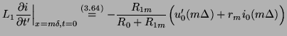
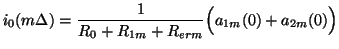
Thus, for initialization, equating the voltages in (3.88) and (3.87), we must have

$$-\frac{R_{1m}(R_{1m}+R_{0}+R_{erm})}{R_{1m}+R_{0}}\left(u_{0}'(m\Delta)+R_{erm}i_{0}(m\Delta)\right) = (R_{0}+R_{er})a_{1m}(0)-R_{1}a_{2m}(0)$$

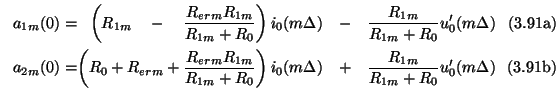
This requirement, along with (3.86) fully specifies the initial values of the wave variables at the left adaptor. We thus have

We note that $u_{0}'(m\Delta)$ may be obtained from the initial voltage distribution $u_{0}(x)$ by any reasonable (i.e., consistent) approximation to the spatial derivative.

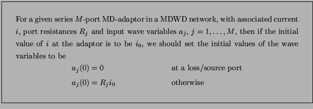
It is important to recognize that for constant $v_{0}$, we have

$$\lim_{\Delta\rightarrow 0}a_{1m}(0) = R_{1m}i_{0}(m\Delta)\hspace{0.5in}\lim_{\Delta\rightarrow 0}a_{2m}(0)= R_{0}i_{0}(m\Delta)$$

These values occur in the same ratio as those of an eigenvector of the scattering matrix for the left series adaptor. In particular, they follow the distribution of the principal eigenvector (i.e., the unique eigenvector whose elements are all of the same sign) of the scattering matrix. Thus the proper setting for the initial conditions (except at the loss port) should be aligned with the dominant mode of the numerical scheme in this limit (and the fraction of the initial energy injected into the parasitic modes will vanish)--see §3.9.2 for a discussion of parasitic modes in this particular system. We also suggest the following very simple ``rule of thumb'' for setting initial conditions:

This rule is to be interpreted in a distributed sense, i.e., it holds for every instance of an adaptor on the numerical grid. A similar rule holds for a parallel adaptor. These settings ignore spatial derivative information, but give a simple way of proceeding in general, especially during the first stages of programming and debugging, and are correct (to first order) in the limit as $\Delta$ approaches 0. If losses are large, though, one may prefer to use exact conditions like (3.89). This rule applies regardless of the number of dimensions of the problem (but may need to be amended if sources or reflection-free ports are present).