Digital Waveguide Networks

• Networks made up of connections of transmission-line like ``unit element'' filters, connected at scattering junctions.
  
  
  
• Originally conceived as a stable means of doing artificial reverberation, and modelling room acoustics.
• Impedances as well as line lengths may be time-varying, (audio effects, such as chorusing, flanging, etc.)
• Same passivity properties as circuit-based method (under finite arithmetic as well).
• a different point of view from the multi-D circuits: Begin in a discrete setting, no spectral mapping is used (explicitly).
• when applied to E+M problems, is roughly equivalent to TLM (Transmission Line Matrix method).

The Bidirectional Delay Line

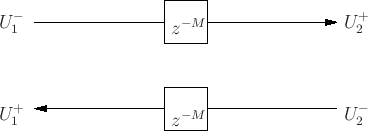
The central element in a digital waveguide network is a bidirectional delay line.

A bidirectional delay line has associated with it

• an impedance $Z>0$ ( $Y=\frac{1}{Z}$ is the admittance
• a delay (usually an integer $M\geq 1$ ) number of samples), same in both directions.

• two incoming and outgoing (voltage) wave variables
• (optional) a physical length.

can be considered a discrete time lossless (LBR) two-port.(Indeed, it is included among the original wave digital filtering elements).

If the delay line pair has a physical length $\Delta$ associated with it, then the two wave variables may be interpreted as travelling wave components which solve the 1D wave equation, where the speed is $c=\Delta/T$ , and $T$ is the sample period.

Traveling Wave Variables

We can define a related set of wave variables (current) in the bidirectional delay line by

$$I_{j}^{+} = \frac{1}{Z}U_{j}^{+}$$

$$I_{j}^{-} = -\frac{1}{Z}U_{j}^{-}$$

for $j=1,2$ .

• sign inversion of incoming current wave with respect to outgoing (not left/right, but could be defined this way).
• current waves are auxiliary; need them only to define scattering junctions (not stored variables).

``Physical'' voltages and currents at the endpoints of the delay line pair:

$$U_{j} = U_{j}^{+}+U_{j}^{-}$$

$$I_{j} = I_{j}^{+}+I_{j}^{-}$$

for $j=1,2$ .

• A different formulation from MD wave digital filters: wave variables are instantaneously related to physical quantities (not to derivatives of them)

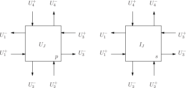
Scattering Junctions

Scattering Junctions (series and parallel) are defined identically to the WDF case.

$$U_{j}^{-} = U_{j}^{+} -\frac{2Z_{j}}{\sum_{j=1}^{k}Z_{j}}\sum_{j=1}^{k}U_{j}^{+}, m=1\hdots k {\mbox {\rm Series Connection}}$$

$$U_{j}^{-} = -U_{j}^{+} +\frac{2}{\sum_{j=1}^{k}Y_{j}}\sum_{j=1}^{k}Y_{j}U_{j}^{+}, m=1\hdots k {\mbox {\rm Parallel Connection}}$$

Comments

• Passivity follows from power conservation at the junctions (Kirchoff's Laws) and LBR property of delay lines. No need to invoke MD-passivity, since we are dealing with, in a sense, lumped elements (unit element filters).
• Passivity under coefficient and signal truncation follows just as in WDF case.
• Generalizations include:
  • Power-normalization of waves (as per WDFs)

  • allowing $Z$ to be time-varying. Still passive, if power-normalized variables are used. (audio effects algorithms)
  • non-integer (and also posibly time-varying) delay line lengths. (audio effects algorithms)
  • delays can be replaced by arbitrary bounded-real functions of $z^{-1}$ (dispersion).
  • vector-valued signals. For an $n$ -component ``waveguide'', we now require:

    $n\times n$ matrix impedance ${\bf Z}$ , with $Z>0$ . $2n\times 2n$ matrix reflectance ${\bf S}$ , ${\bf S}$ paraunitary. (comes in handy for solids, also as framework for treating TLM ``super-symmetric condensed node'')

1D Transmission Line Revisited

The lossless source-free 1D transmission line equations are

$$l\frac{\partial i}{\partial t} + \frac{\partial u}{\partial x} =$$ 0

$$c\frac{\partial u}{\partial t} + \frac{\partial i}{\partial x} =$$ 0

Can apply centered differences over a uniform grid:

$$I_{i+\frac{1}{2}}(n+{\textstyle \frac{1}{2}}) - I_{i+\frac{1}{2}}(n-{\textstyle \frac{1}{2}}) + \frac{1}{v_{0} \bar{l}_{i+\frac{1}{2}}}\left(U_{i+1}(n)-U_{i}(n)\right) = 0$$

$$U_{i}(n) - U_{i}(n-1) + \frac{1}{v_{0} \bar{c}_{i}}\left(I_{i+\frac{1}{2}}(n-{\textstyle \frac{1}{2}})-I_{i-\frac{1}{2}}(n-{\textstyle \frac{1}{2}})\right) = 0$$

$$U_{i}(n)\qquad {\rm approximates}\qquad u(i\Delta,nT)$$

$$I_{i+\frac{1}{2}}(n+\frac{1}{2})\qquad {\rm approximates}\qquad i((i+\frac{1}{2})\Delta, (n+\frac{1}{2})T)$$

• Grid variables are staggered in time and space (Yee, FDTD).

Constant Parameters

If $l$ and $c$ are constant, and we choose $v_{0}=\sqrt{\frac{1}{lc}}$ , then the difference equations simplify to a single equation in the voltages alone:

$$U_{i}(n+1) + U_{i}(n-1) = U_{i+1}(n)+U_{i-1}(n)$$

Just solving the wave equation, at the CFL limit.

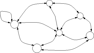
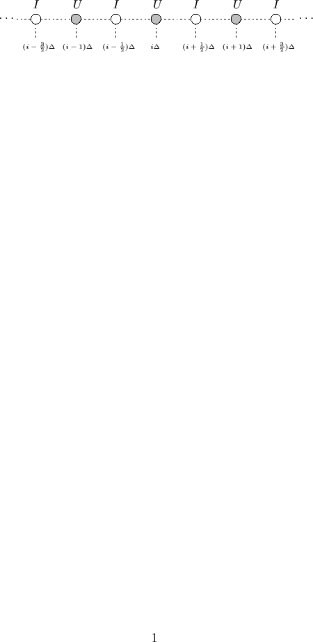
Consider a chain of bidirectional delay lines, of length $\Delta$ , and operating at time step $T$ connected by parallel junctions:

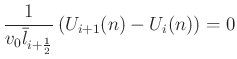
• Junction voltages solve the wave equation at CFL, if all impedances are identical (no scattering)

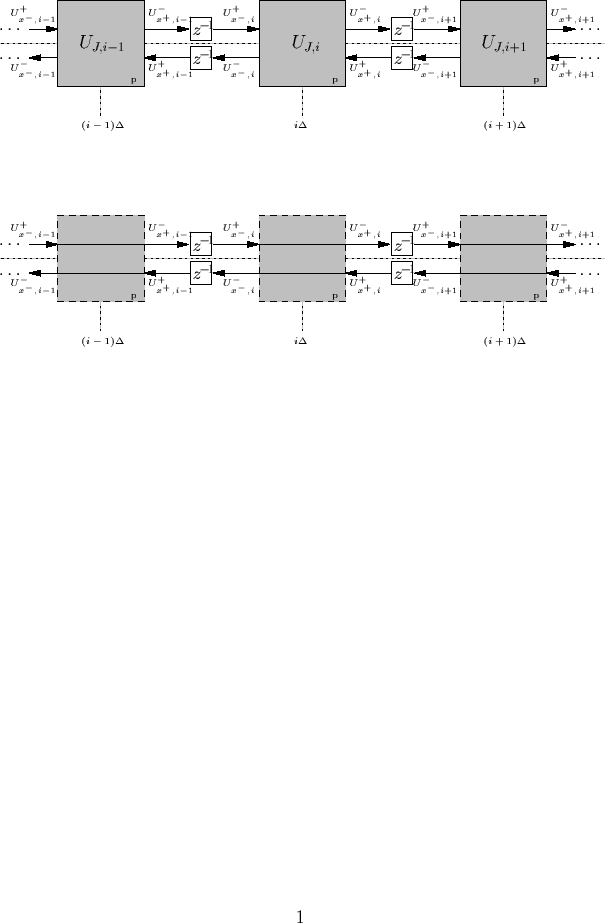
An Interleaved Mesh

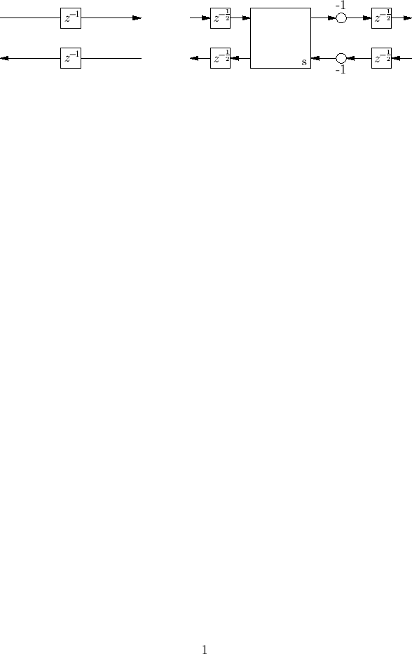
Notice that it is possible to split a bidirectional delay line in the following way:

• Now have two half-sample, half-length delay lines of equal impedance (series junction functions, for the moment,as merely a sign inverter).
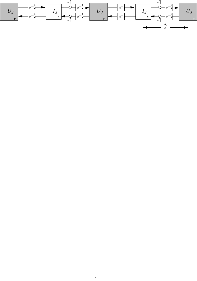
• Can employ this identity in the previous structure:

• Solves constant-parameter Transmission Line Equations, at CFL, on interleaved grid, if we choose $Z=\sqrt{\frac{l}{c}}$ for all subsections.
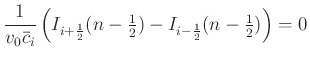
• Junction currents at series junctions give physical current.

Varying Material Parameters

Now we have $l(x)$ and $c(x)$ .

• Expect dispersion (scattering due to varying line impedance) Natural fix: Delay line impedances should be different.
• Local propagation speed, $\sqrt{\frac{1}{lc}}$ also varies Fix: Insert passive ``storage'' registers at every junction, in order to slow down local propagation speed in mesh.

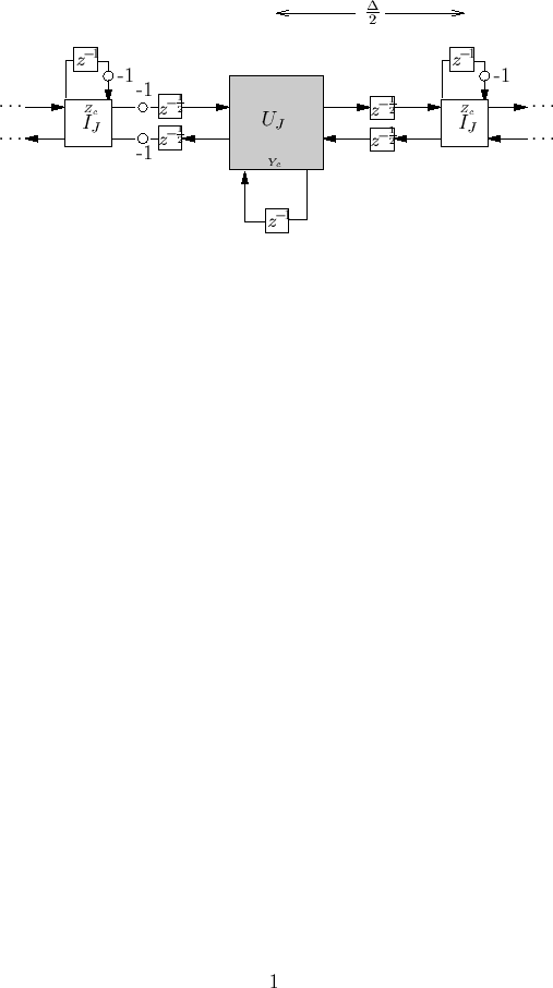
Examine a mesh of the following form:

• will solve T-line equations if line impedances chosen properly
• Get a family of difference methods, each with different stability properties.
• stability constraints derive from positivity condition on impedances (as per WDFs).

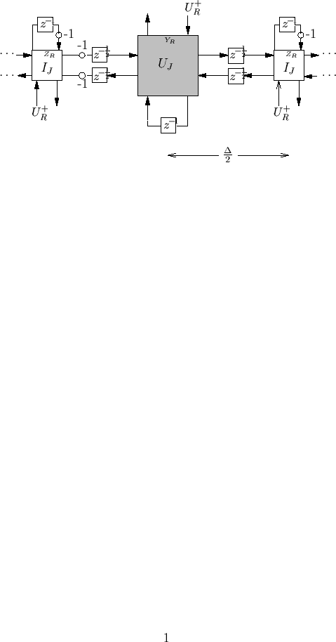
Losses and Sources

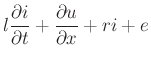
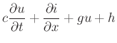
The full Transmission Line Equations are, including losses (resistive, and shunt conductive):

$$l\frac{\partial i}{\partial t}+\frac{\partial u}{\partial x}+ri+e =$$ 0

$$c\frac{\partial u}{\partial t}+\frac{\partial i}{\partial x}+gu+h =$$ 0

Can treat this by adding a ``resistive source'' (analogous to WDF counterpart) at every junction:

Simplifies considerably in certain cases...