The Gas Dynamics Equations

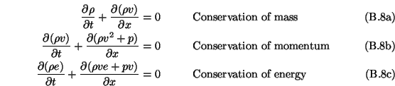
The behavior of a lossless one-dimensional fluid is described by the following set of conservation equations, also known as Euler's Equations:

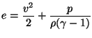
where $\rho(x,t)$ is density, $v(x,t)$ is volume velocity, $p(x,t)$ is absolute pressure, and $e(x,t)$ is total energy, internal plus kinetic. The three equations are not complete without a constitutive relation among the four dependent variables. The WDF people, in their treatment of hydrodynamics [16] often leave out the energy equation and make an assumption of the type $p = G(\rho)$, which essentially reduces system (B.9) to a two-variable system (in $\rho$ and $v$). For gas dynamics, we assume polytropic gas behavior [181]:

$$e = \frac{v^{2}}{2} + \frac{p}{\rho (\gamma-1)}$$ (B.10)

where $\gamma>1$ is a constant which follows directly from thermodynamics (it is equal to the ratio of specific heats [203]).

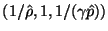
Before proceeding any further, we mention the scaling of the dependent variables [16,49]; this is done, as in the linear problems discussed in Chapters 3 and 5, in order to optimize the stability condition on the resulting network. The variables are scaled as

$$\hat{v} = \frac{v}{v_{0}}\hspace{0.2in} \hat{p} = \frac{p}{p_{0}}\hspace{0.2in} \hat{\rho} = \frac{\rho v_{0}^{2}}{p_{0}}$$ (B.11)

The parameters $v_{0}$ and $p_{0}$ have dimensions of velocity and pressure, respectively, and nondimensionalize the system. $v_{0}$ will again become the space-step/time-step ratio in the numerical simulation routine, and $p_{0}$ plays a role similar to that of $r_{0}$ in the (1+1)D transmission line problem as discussed in §3.7 and follows directly from physical considerations.

Using the energy density definition (B.10), system (B.9) can be written in non-conservative [203] form (after some tedious algebraic manipulations) as

$$\begin{bmatrix}1&0&0\\ 0&\hat{\rho}&0\\ 0&0&1\\ \end{bmatrix} \fr... ...tial x}\begin{bmatrix}\hat{\rho}\\ \hat{v}\\ \hat{p}\\ \end{bmatrix}=\mathbf{0}$$

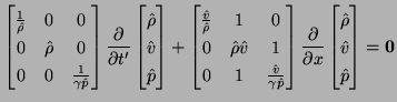
The problem here is that this system is not, in its present form, suitable for a circuit representation involving reciprocal elements. Although it is not explicitly stated anywhere in the literature, the solution of Fettweis et al. has been to scale system (B.9) by left multiplication by the matrix diag $(1/\hat{\rho}, 1, 1/(\gamma \hat{p}))$ (though as previously mentioned, they work with the two-variable hydrodynamics system, or its analogues in higher dimensions). The scaled system takes the form:

$$\begin{bmatrix}\frac{1}{\hat{\rho}}&0&0\\ 0&\hat{\rho}&0\\ 0&0&\f... ...tial x}\begin{bmatrix}\hat{\rho}\\ \hat{v}\\ \hat{p}\\ \end{bmatrix}=\mathbf{0}$$ (B.12)

While this scaling does not change smooth solutions to system (B.9), problems may occur if shocks are anticipated [181]. Such so-called weak solutions [181] to system (B.9) (solutions involving discontinuities which must be described using the integral formulation of (B.9)) are not necessarily preserved under such a scaling. Entropy variables, to be briefly mentioned in §B.3.3, allow a potential means of avoiding these difficulties.

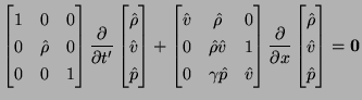
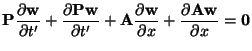
Finally, by employing the conservation of mass equation to simplify the other equations, the scaled system (B.12) can be written in skew-selfadjoint form [181] as:

$${\bf P}\frac{\partial {\bf w}}{\partial t'}+ \frac{\partial {\bf ... ...rac{\partial {\bf w}}{\partial x}+\frac{\partial {\bf Aw}}{\partial x} = {\bf0}$$ (B.13)

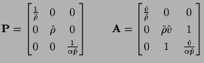
where the symmetric matrices ${\bf P}$ and ${\bf A}$ are defined by

$${\bf P} = \begin{bmatrix}\frac{1}{\hat{\rho}}&0&0\\ 0&\hat{\rho}&... ...0\\ 0&\hat{\rho} \hat{v}&1\\ 0&1&\frac{\hat{v}}{\alpha \hat{p}}\\ \end{bmatrix}$$

and ${\bf w}$ is the state, $[\hat{\rho}, \hat{v}, \hat{p}]^{T}$, and $\alpha = \frac{2\gamma}{\gamma-1}>0$. ${\bf P}$, in addition, will be positive definite if the density and pressure are positive everywhere. The significance of this skew-selfadjoint form can be seen by taking the inner product of (B.13) with ${\bf w}$, in which case we get

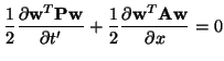$$\frac{1}{2}\frac{\partial {\bf w}^{T}{\bf Pw}}{\partial t'} + \frac{1}{2}\frac{\partial {\bf w}^{T}{\bf Aw}}{\partial x} = 0$$ (B.14)

For the Cauchy problem (i.e., the problem is defined over the entire $x$ axis, so boundary conditions are effectively ignored), we may integrate over the domain to get

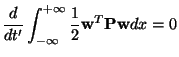$$\frac{d}{dt'}\int_{-\infty}^{+\infty}\frac{1}{2}{\bf w}^{T}{\bf Pw}dx = 0$$ (B.15)

and thus 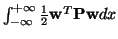$\int_{-\infty}^{+\infty}\frac{1}{2}{\bf w}^{T}{\bf Pw}dx$ is the global conserved quantity. It can be seen, by comparison between (B.14) and (B.15) with (3.3) and (3.5) (in the lossless case), that this skew-selfadjointness property is the natural extension of symmetric hyperbolicity to the nonlinear case. It is interesting that the generalized definitions of the inductor and capacitor, as per (B.1) and (B.3), are completely commensurate; we will see this in the next section. The theory of skew-selfadjoint forms has recently seen quite a bit of activity, in particular with regard to so-called entropy variables [68,84,95,180,181,182,183], which we will look at briefly in §B.3.3.