MDKC and MDWDF for the Gas Dynamics Equations

It is particularly easy to see the form of the MDKC for the gas dynamics equations in the scaled form of (B.13). Applying the usual coordinate transformation (3.18), (B.13) becomes

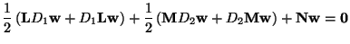$$\frac{1}{2}\left({\bf L}D_{1}{\bf w}+ D_{1}{\bf L}{\bf w}\right)+... ...c{1}{2}\left({\bf M}D_{2}{\bf w}+ D_{2}{\bf M}{\bf w}\right) + {\bf Nw}= {\bf0}$$ (B.16)

with

$${\bf L} = \begin{bmatrix}\frac{1+\hat{v}}{\hat{\rho}}&0&0\\ 0&\ha... ...t{\rho}(1-\hat{v})-1&0\\ 0&0&\frac{1-\hat{v}}{\alpha \hat{p}}-1\\ \end{bmatrix}$$

and

$${\bf N} = \begin{bmatrix}0&0&0\\ 0&D_{1}+D_{2}&D_{1}-D_{2}\\ 0&D_{1}-D_{2}&D_{1}+D_{2}\\ \end{bmatrix}$$

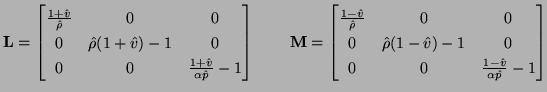
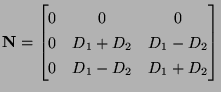
The MDKC is shown in Figure B.2(a), where the inductances can be read directly from the entries of ${\bf L}$, ${\bf M}$ and ${\bf N}$. ${\bf L}$ and ${\bf M}$ represent the inductances in the three loops in directions $t_{1}$ and $t_{2}$ respectively, and ${\bf N}$ gives the coupling between the second and third loops (notice that it can be realized as a simple linear and shift-invariant Jaumann two-port, just as in the linear systems of Chapter 3). The first loop, with current $\hat{\rho}$ is decoupled from the other two, although the inductances in this loop are dependent on $\hat{v}$.

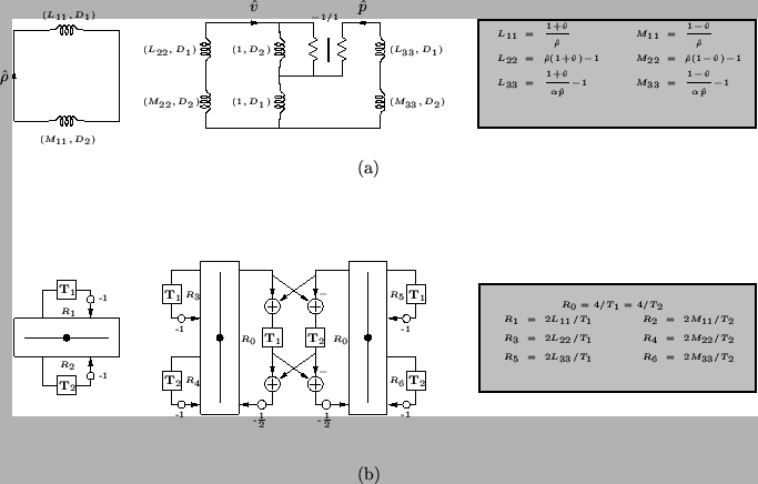
The MDWD network follows immediately, and is shown in Figure B.2(b). It should be kept in mind that the port resistances at the adaptors are now functions of the dependent variables (the currents in the MDKC), and thus of the wave variables themselves. In a given updating cycle, the current values of the port resistances must be determined from the incoming waves. Due to the fact that power normalized variables are used, this leads to a system of coupled nonlinear algebraic equations (three, one for each adaptor) to be solved at every grid point, and at every time step.

Figure B.2: The (1+1)D gas dynamics system-- (a) MDKC and (b) MDWD-network.

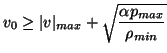
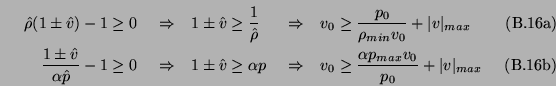
Passivity is contingent upon the positivity of all the inductances in the network; this is essentially a condition on the positivity of the diagonal matrices ${\bf L}$ and ${\bf M}$. Proceeding down the diagonals, this requirement on the first elements leads to the natural condition

$$1\pm \hat{v} \geq 0 \hspace{0.3in}\Rightarrow\hspace{0.3in} v_{0}\geq \vert v\vert _{max}$$

where $\vert v\vert _{max}$ is the maximum value that $\vert v\vert$ will take over the problem domain, and during the simulation period. We have also assumed that $\rho$ remains positive, and used the definition of the scaled quantity $\hat{v}$ from (B.11). The conditions on the other elements of ${\bf L}$ and ${\bf M}$ are more strict. We get

where $\rho_{min}$ and $p_{max}$ are, respectively, the minimal value of $\rho$ and the maximum value of $p$ that will be encountered in the problem space. These quantities, as well as $\vert v\vert _{max}$ must be estimated a priori. It is also worth mentioning that for the above reasoning to be valid, it has been assumed that $\rho$ and $p$ will remain positive, and that $\rho$ is bounded from below. Although this has not been mentioned in the literature, there does not appear to be any assurance that these assumptions will remain valid during the course of a simulation.

We still have one degree of freedom left, namely the value of the parameter $p_{0}$. An optimal setting is easily shown to be

$$p_{0} = v_{0}\sqrt{\alpha p_{max}\rho_{min}}$$

in which case the two bounds on $v_{0}$ from (B.17) coalesce, giving

$$v_{0} \geq \vert v\vert _{max} + \sqrt{\frac{\alpha p_{max}}{\rho_{min}}}$$