Burger's Equation

A simple nonlinear PDE which is often used as a model problem for fluid dynamical systems is given by the inviscid Burger's equation [82]:

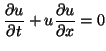$$\frac{\partial u}{\partial t} + u\frac{\partial u}{\partial x} = 0$$ (B.4)

It is similar in form to the advection equation mentioned in §3.6, and as we will see, its circuit representation is identical. The problem is assumed to be defined for $x\in \mathbb{R}$, $t\geq 0$. $u$ can be considered to be a current, as before, through a single loop, and Kirchoff's Voltage Law around the loop will give (B.4). The question however, is of the type of circuit elements to be included in this loop; clearly they must be nonlinear, and certainly reactive as well. We note that the viscous form of Burger's equation was approached in this way in [202].

Using coordinate transformation (3.18), (B.4) can be rewritten as

$$\left(\frac{v_{0}+u}{\sqrt{2}}\right)\frac{\partial u}{\partial t_{1}}+\left(\frac{v_{0}-u}{\sqrt{2}}\right)\frac{\partial u}{\partial t_{2}} = 0$$

Assuming that the solution is differentiable, this can be rewritten as

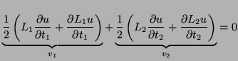$$\underbrace{\frac{1}{2}\left(L_{1}\frac{\partial u}{\partial t_{1... ...l u}{\partial t_{2}}+\frac{\partial L_{2}u}{\partial t_{2}}\right)}_{v_{2}} = 0$$ (B.5)

where

$$L_{1} = \frac{1}{\sqrt{2}}\left(v_{0} + \frac{2}{3}u\right)\hspace{0.5in} L_{2} = \frac{1}{\sqrt{2}}\left(v_{0} - \frac{2}{3}u\right)$$ (B.6)

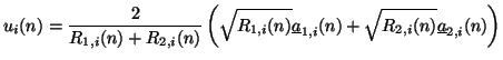
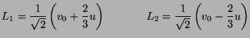
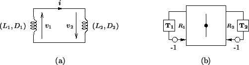
Thus Burger's equation, in the form of (B.5), can be interpreted as a series combination of two nonlinear inductances, as shown in Figure B.1(a). The resultant MDWD network, with port resistances

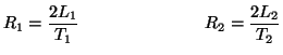$$R_{1} = \frac{2L_{1}}{T_{1}}\hspace{1.0in}R_{2} = \frac{2L_{2}}{T_{2}}$$ (B.7)

appears in Figure B.1(b). We emphasize that this network is passive only if power-normalized wave variables are employed.

Figure B.1: The (1+1)D inviscid Burger's equation-- (a) MDKC and (b) MDWD network.

The positivity condition on these inductances now depends on the solution itself, $u$, and we must have

$$v_{0} \geq \frac{2}{3}\max_{x\in \mathbb{R},t\geq 0}\vert u\vert$$

An a priori estimate of $\max_{x\in \mathbb{R},t\geq 0}\vert u\vert$ must be available; this is a consistent feature of all the circuit-based methods (and, it would seem, any explicit method) for the fluids systems that we will examine presently.

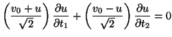
Let us now examine the scattering operation. First choose $T_{1}=T_{2}=\sqrt{2}\Delta$, so that the current grid function for the current at location $x=i\Delta$ and $t = nT$ can be written as $u_{i}(n)$. The two power-normalized input wave variables entering the adaptor at the same location and time step are $\underline{a}_{1,i}(n)$ $\underline{a}_{2,i}(n)$, and we have

$$u_{i}(n) = \frac{2}{R_{1,i}(n)+R_{2,i}(n)}\left(\sqrt{R_{1,i}(n)}\underline{a}_{1,i}(n)+\sqrt{R_{2,i}(n)}\underline{a}_{2,i}(n)\right)$$

which, from (B.6) and (B.7), and using $T_{1}=T_{2}=\sqrt{2}\Delta$ and $v_{0} = \Delta/T$ can be rewritten as

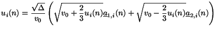$$u_{i}(n) = \frac{\sqrt{\Delta}}{v_{0}}\left(\sqrt{v_{0}+\frac{2}{... ...rline{a}_{1,i}(n)+\sqrt{v_{0}-\frac{2}{3}u_{i}(n)}\underline{a}_{2,i}(n)\right)$$ (B.8)

This is precisely the nonlinear algebraic equation which is to be solved (in $u_{i}(n)$); once $u_{i}(n)$ is determined, then so are the port resistances, and the output wave variables $\underline{b}_{1,i}(n)$ and $\underline{b}_{2,i}(n)$ can be obtained through scattering as per (2.33). As mentioned before, it is not at all clear from the form of (B.8) whether a solution exists and is unique. We note, however, that we (and others [16,70]) have successfully programmed simulations for the gas dynamics equations (see next section), using simple iterative methods to solve the nonlinear algebraic systems; the results would appear to be in accord with published simulation results using differencing methods [171].