Nonlinear Circuit Elements

It should be clear that in order to build circuit models for nonlinear systems of PDEs, we will need nonlinear distributed circuit elements. Nonlinear resistances are simple to model; a voltage-current relation of the form

$$v = iR$$

will correspond to a passive resistor as long as $R$ is positive, regardless of its dependence on $v$, $i$, or the independent variables of the problem. The definitions of transformers and gyrators also remain unchanged in the nonlinear case; the turns ratio or gyration coefficient may have any dependence without affecting losslessness.

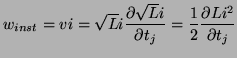
Nonlinear reactances require only a slightly more involved treatment. Recall the generalized definition of the inductor as given in (3.42):

$$v = \sqrt{L}\frac{\partial}{\partial t_{j}}\left(\sqrt{L}i\right)... ...(L\frac{\partial i}{\partial t_{j}} + \frac{\partial Li}{\partial t_{j}}\right)$$ (B.1)

Here again, $t_{j}$ is some coordinate defined by a transformation such as (3.15) or (3.21). The instantaneous absorbed power density will be

$$w_{inst} = vi = \sqrt{L}i\frac{\partial \sqrt{L}i}{\partial t_{j}} = \frac{1}{2}\frac{\partial Li^{2}}{\partial t_{j}}$$

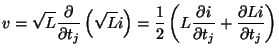
and the element can be considered to be lossless as per the definition of (3.28) provided the stored energy flux ${\bf E}$ is defined to be

$${\bf E} = \frac{1}{2}Li^{2}{\bf e}_{j}$$

where ${\bf e_{j}}$ is a unit vector in the direction $t_{j}$. This is the same as the definition in the linear case, from (3.35). Here, $L$ is constrained to positive, but may be be a function (smooth) of any of the dependent or independent variables in the problem. This losslessness is reflected in the MDWD one-port; if the port resistance is chosen to be $R=2L/T_{j}$, for some step-size $T_{j}$ in direction $t_{j}$, then in terms of power-normalized waves $\underline{a}$ and $\underline{b}$ (see §2.3.2), the one-port is defined, at a grid point with coordinates ${\bf t}$, by

$$\underline{b}({\bf t}) = -\underline{a}({\bf t}-{\bf T}_{j})$$ (B.2)

for a vector shift ${\bf T}_{j} = T_{j}{\bf e}_{j}$, just as in the linear case. It is important to mention that for a nonlinear problem, it is essential to use power-normalized waves, because passivity is not guaranteed otherwise [16]. (The reason for this should be clear from the discussion in §3.5.1; we cannot obtain a wave relation such as (B.2) in terms of voltage wave variables because the differential operator does not necessarily commute with the inductance.)

A nonlinear capacitor can be similarly defined, by

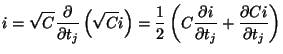$$i = \sqrt{C}\frac{\partial}{\partial t_{j}}\left(\sqrt{C}i\right)... ...(C\frac{\partial i}{\partial t_{j}} + \frac{\partial Ci}{\partial t_{j}}\right)$$ (B.3)

for some capacitance $C$, which again may have arbitrary smooth functional dependence; if $C$ is always positive, then the capacitance is lossless.

Notice that for all practical purposes, the nonlinear character of any one of these elements is essentially transferred to the port resistances of the adaptor to which it is connected; the wave digital elements themselves are identical to their linear counterparts. As long as the circuit element values remain positive, then so do the port resistances, and an adaptor scattering matrix will be forced to be orthogonal (see §2.3.5), and can be interpreted in terms of rotations and reflections. The problem, then, is in determining the scattering matrix, which, though orthogonal, may be dependent on the input waves; a system of nonlinear algebraic equations results. This problem is usually solved in practice using iterative methods, but existence and uniqueness of such a solution are matters which have not been broached in any detail (and should be). These systems of equations are usually small, however, and can be solved separately at a any given grid point.