Next |
Prev |
Top
|
Index |
JOS Index |
JOS Pubs |
JOS Home |
Search
Introduction to Laplace Transform Analysis
The one-sided Laplace transform of a signal  is defined
by
is defined
by
where  is real and
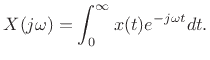 is a complex variable. The
one-sided Laplace transform is also called the unilateral
Laplace transform. There is also a two-sided, or
bilateral, Laplace transform obtained by setting the lower
integration limit to
is a complex variable. The
one-sided Laplace transform is also called the unilateral
Laplace transform. There is also a two-sided, or
bilateral, Laplace transform obtained by setting the lower
integration limit to  instead of 0. Since we will be
analyzing only causalD.1 linear systems using the Laplace transform, we can use
either. However, it is customary in engineering treatments to use the
one-sided definition.
instead of 0. Since we will be
analyzing only causalD.1 linear systems using the Laplace transform, we can use
either. However, it is customary in engineering treatments to use the
one-sided definition.
When evaluated along the  axis (i.e.,
  ), the
Laplace transform reduces to the unilateral Fourier transform:
), the
Laplace transform reduces to the unilateral Fourier transform:
The Fourier transform is normally defined bilaterally (
 above), but for causal signals
, there is no
difference. We see that the Laplace transform can be viewed as a
generalization of the Fourier transform from the real line (a simple
frequency axis) to the entire complex plane. We say that the Fourier
transform is obtained by evaluating the Laplace transform along the
above), but for causal signals
, there is no
difference. We see that the Laplace transform can be viewed as a
generalization of the Fourier transform from the real line (a simple
frequency axis) to the entire complex plane. We say that the Fourier
transform is obtained by evaluating the Laplace transform along the
 axis in the complex
  plane.
An advantage of the Laplace transform is the ability to transform signals which
have no Fourier transform. To see this, we can write the Laplace
transform as
Thus, the Laplace transform can be seen as the Fourier transform of an
exponentially windowed input signal.
For  (the so-called ``strict right-half plane'' (RHP)), this
exponential weighting forces the Fourier-transformed signal toward
zero as
(the so-called ``strict right-half plane'' (RHP)), this
exponential weighting forces the Fourier-transformed signal toward
zero as
 . As long as the signal
does not increase
faster than
. As long as the signal
does not increase
faster than 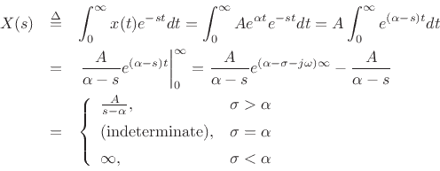 for some
  , its Laplace transform will exist for all
 . We make this more precise in the next section.
Subsections
Next |
Prev |
Top
|
Index |
JOS Index |
JOS Pubs |
JOS Home |
Search
[How to cite this work] [Order a printed hardcopy] [Comment on this page via email]


![$\displaystyle X(s) = \int_0^\infty x(t) e^{-(\sigma + j\omega)t} dt
= \int_0^\infty \left[x(t)e^{-\sigma t}\right] e^{-j\omega t} dt .
$](img1685.png)