Scattering Networks for the Navier System

Nitsche has represented this system as an MDKC in [131]. Choosing current-like variables

$$(i_{1},i_{2},i_{3},i_{4},i_{5},i_{6},i_{7},i_{8},i_{9}) = (v_{x},... ...sigma_{yy},r_{1}\sigma_{zz},r_{2}\sigma_{xy},r_{2}\sigma_{xz},r_{2}\sigma_{yz})$$

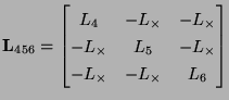
he derived an MDKC for the Navier system, which we have reproduced (with some minor changes) at top in Figure 5.25, where coordinates defined by the transformation matrix (3.24) have been used. Notice that again, because ${\bf P}$ is not diagonal, the time derivatives of the components $\sigma_{xx}$, $\sigma_{yy}$ and $\sigma_{zz}$ are coupled. In the circuit representation, this is represented by a three-port coupled inductance of the form of (2.48), with a matrix inductance ${\bf L}_{456}$ defined by

$${\bf L}_{456} = \begin{bmatrix}L_{4}&-L_{\times}&-L_{\times}\\ -L_{\times}&L_{5}&-L_{\times}\\ -L_{\times}&-L_{\times}&L_{6}\\ \end{bmatrix}$$

where the inductances $L_{4}$, $L_{5}$, $L_{6}$ and $L_{\times}$ appear in the figure.

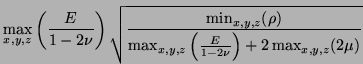
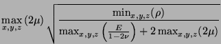
The positivity condition on the inductances $L_{1}$, $L_{2}$, $L_{3}$, $L_{7}$, $L_{8}$ and $L_{9}$, as well as a positive definiteness condition on the matrix ${\bf L}_{456}$ gives, as optimal choices of the parameters $r_{1}$ and $r_{2}$,

$$r_{1} = \max_{x,y,z}\left(\frac{E}{1-2\nu}\right)\sqrt{\frac{\min_{x,y,z}(\rho)}{\max_{x,y,z}\left(\frac{E}{1-2\nu}\right)+2\max_{x,y,z}(2\mu)}}$$

$$r_{2} = \max_{x,y,z}\left(2\mu\right)\sqrt{\frac{\min_{x,y,z}(\rho)}{\max_{x,y,z}\left(\frac{E}{1-2\nu}\right)+2\max_{x,y,z}(2\mu)}}$$

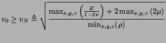
and a bound on $v_{0}$,

$$v_{0}\geq v_{N}\triangleq\sqrt{\frac{\max_{x,y,z}\left(\frac{E}{1-2\nu}\right)+2\max_{x,y,z}\left(2\mu\right)}{\min_{x,y,z}(\rho)}}$$

When the material parameters are constant, $v_{N}$ reduces to

$$v_{N} = \sqrt{\frac{3(\lambda+2\mu)}{\rho}} = \sqrt{3}\gamma_{N, max}^{g}$$

A modified MDKC is shown at top in Figure 5.26, where velocities are treated as currents, and stresses as voltages; as such, the coupled inductance in Figure 5.25 has become a coupled capacitance. This network may be discretized in a way very similar to the network for Maxwell's Equations, as described in §4.10.6. Under the spectral mappings defined by (4.112) (with step sizes of $T_{j} = \Delta/2$, $j=1,\hdots,6$), the connecting LSI two-ports decompose into series/parallel connections of multidimensional unit elements. The one-port inductances and capacitances, as well as the coupled capacitance are discretized using the trapezoid rule, with a step size of $T_{7} = \Delta$. The resulting multidimensional DWN is shown at bottom in Figure 5.26, and the interleaved computational grid in Figure 5.27 (which is very similar to the grid for the DWN for Maxwell's Equations, as shown in Figure 4.55).