Boundary Conditions

The simplest boundary conditions for the Navier system are of the free type, i.e., all stresses normal to the boundary are zero [77]. For a ``bottom'' boundary $z=0$, these conditions can be written as

$$\sigma_{xz} = \sigma_{yz} = \sigma_{zz} = 0$$ (5.57)

This condition is lossless and of the form of (3.8).

Figure 5.25: MDKC and MDWD network for the Navier system.

Figure 5.26: Modified MDKC and multidimensional DWN for the Navier system.

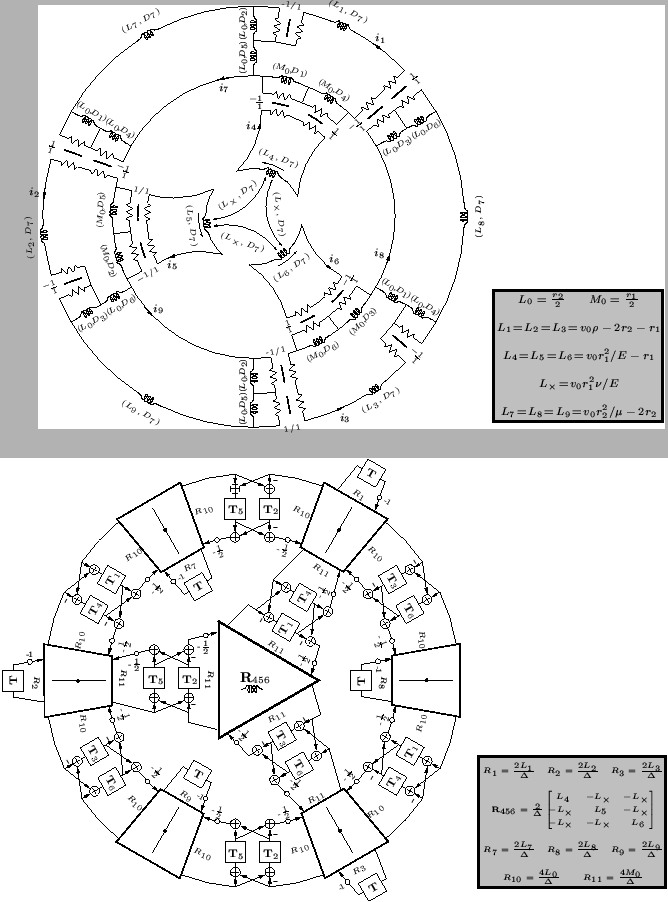
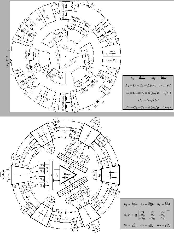
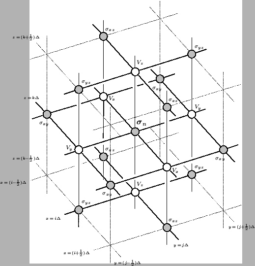
Considering the DWN shown at bottom in Figure 5.26, and the associated computational grid shown in Figure 5.27, it is easy to see that in this case, it best to arrange the grid such that parallel junctions (at which approximations to $\sigma_{xz}$ and $\sigma_{yz}$ are calculated) lie on this bottom boundary. The first two of conditions (5.55) can be ensured by short-circuiting the parallel junctions. As a result, the remaining series junctions on the boundary (at which approximations to $v_{z}$ are calculated) are decoupled from the parallel junctions, and it remains only to set a self-loop impedance at these junctions so as to approximate the condition $\sigma_{zz} = 0$. We leave the determination of these self-loop impedances as an exercise to the reader.

Figure 5.27: Computational grid for the DWN for Navier's system; stresses and velocities are calculated at alternating multiples of $T/2$, and at alternating grid locations. In the DWN implementation, waveguide connections (of delay length $T/2$) between series junctions (white) and parallel junctions (grey) are shown as dark lines; waveguide sign inversions and self-loops are not shown here. At the center grid point, a vector parallel junction calculates the vector $\sigma$ $_{n} = (\sigma_{xx}, \sigma_{yy}, \sigma_{zz})$ of normal stresses.