Scattering Networks for Maxwell's Equations

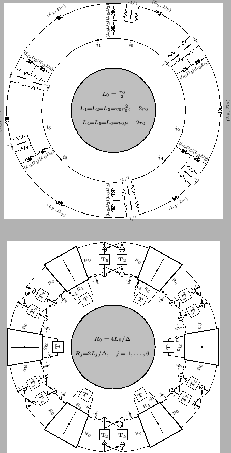
This system has been represented by an MDKC in [50,131], where the coordinate transformation defined by (3.24) has been employed, and the current variables are defined by

$$(i_{1},i_{2},i_{3},i_{4},i_{5},i_{6}) = (E_{x}/r_{0},E_{y}/r_{0},E_{z}/r_{0},H_{x},H_{y},H_{z})$$

for some positive constant $r_{0}$. We have reproduced this MDKC in Figure 4.53. This network can be viewed as two coupled (2+1)D parallel-plate networks (see §3.8), and this is not surprising, given that the (2+1)D parallel-plate system is essentially equivalent to the transverse electric (TE) or transverse magnetic (TM) system alone. The resulting MDWD network is shown, at bottom, in Figure 4.53; here, we have assumed the directional shifts ${\bf T}_{j}$, $j=1,\hdots,7$ to be of length $\Delta$. (And thus $T_{7} = T'= \Delta/v_{0}\triangleq T$.)

Figure 4.53: MDKC and MDWD network for Maxwell's equations (4.110).

The passivity condition is again a condition on the positivity of the network inductances in the MDKC; these values are given in Figure 4.53, and the resulting conditions are

$$v_{0}\geq \frac{2}{r_{0}\epsilon_{min}} \hspace{1.0in} v_{0}\geq \frac{2r_{0}}{\mu_{min}}$$

Under the choice of $r_{0} = \sqrt{\frac{\mu_{min}}{\epsilon_{min}}}$, the stability condition becomes

$$v_{0}\geq\frac{2}{\sqrt{\mu_{min}\epsilon_{min}}}\geq 2\gamma_{Maxwell,max}^{g}$$ (4.128)

with

$$\epsilon_{min} = \min_{x,y,z}\epsilon\hspace{1.0in}\mu_{min} = \min_{x,y,z}\mu$$

and the numerical scheme is passive and hence stable over this range of $v_{0}$.

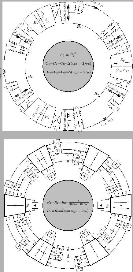
In order to generate a digital waveguide network, we may proceed as for the (1+1)D transmission line and (2+1)D parallel-plate systems discussed in §4.10.3 and §4.10.4, and apply the by now familiar network transformations to yield the modified circuit shown in Figure 4.54. Electric field quantities are now treated as voltages across capacitors, and the six LSI connecting two-ports will all become multidimensional unit elements under the application of alternative spectral mappings.

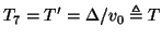
The coordinate transformation from coordinates ${\bf u} = [x,y,z,t]^{T}$ to coordinates ${\bf t} = [t_{1},\hdots,t_{7}]^{T}$ defined by (3.21), using the transformation matrix of (3.24) gives us, in the LSI case, seven frequencies $s_{1},\hdots,s_{7}$. For the connecting two-ports, we may use pairwise spectral mappings defined by

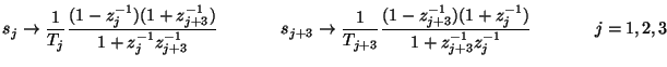$$s_{j}\rightarrow \frac{1}{T_{j}}\frac{(1-z_{j}^{-1})(1+z_{j+3}^{-... ...{(1-z_{j+3}^{-1})(1+z_{j}^{-1})}{1+z_{j+3}^{-1}z_{j}^{-1}}\hspace{0.5in}j=1,2,3$$ (4.129)

where $z_{j}^{-1}$, $j=1,\hdots,6$ corresponds to a unit shift in direction $t_{j}$, and the step-sizes $T_{j}$, $j=1,\hdots,6$ are all chosen equal to $\Delta/2$. For the one-port time inductors and capacitors, we use the trapezoid rule with a step-size of $T_{7} = T' = \Delta$. The resulting multidimensional DWN is shown at bottom in Figure 4.54, and the stability bound is unchanged from (4.111).

Figure 4.54: Modified MDKC and multidimensional DWN for Maxwell's equations (4.110).

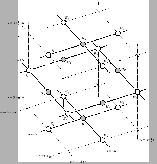
When the spatial dependence is expanded out, we have a DWN operating on an interleaved numerical grid as shown in Figure 4.55, with the electric and magnetic field components calculated at parallel (white) and series (grey) junctions respectively. The connecting waveguide impedances (of delay $T/2$, shown as solid lines) are all equal to $r_{0}$, and the self-loops (of delay $T$, not shown) have impedances $2v_{0}\mu-2r_{0}$ and admittances $2v_{0}\epsilon-2/r_{0}$ at the series and parallel junctions respectively, where these expressions are evaluated at the junction location. It is also possible to derive DWNs of the type I and II forms (see §4.3.6), for which the stability bound is improved to CFL.

Figure 4.55: Computational grid for FDTD applied to Maxwell's equations (4.110); electric and magnetic field quantities are calculated at alternating multiples of $T/2$, and at alternating grid locations. In the DWN implementation, waveguide connections (of delay length $T/2$) between series junctions (grey) and parallel junctions (white) are shown as dark lines; waveguide sign inversions and self-loops are not shown here.

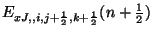
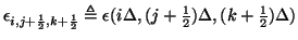
It is easy to verify that this scheme is indeed a scattering form of FDTD. Referring to Figure 4.55, we will have six sets of junction quantities: at the parallel junctions, we will have 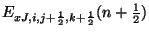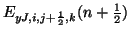$E_{xJ, i,j+\frac{1}{2}, k+\frac{1}{2}}(n+{\textstyle \frac{1}{2}})$, $E_{yJ, i, j+\frac{1}{2}, k}(n+{\textstyle \frac{1}{2}})$ and $E_{zJ, i+\frac{1}{2}, j+\frac{1}{2}, k}(n+{\textstyle \frac{1}{2}})$, and at the series junctions, we will have $H_{xJ, i+\frac{1}{2}, j,k}(n)$, $H_{yJ, i,j+\frac{1}{2},k}(n)$ and $H_{zJ, i,j,k+\frac{1}{2}}(n)$. The indices $i$, $j$, $k$ and $n$ take on integer values. Examine the DWN at a parallel junction with ``voltage'' $E_{xJ,, i,j+\frac{1}{2}, k+\frac{1}{2}}(n+{\textstyle \frac{1}{2}})$. The DWN updates this grid function according to

$$E_{xJ, i, j+\frac{1}{2},k+\frac{1}{2}}(n+{\textstyle \frac{1}{2}}) = E_{xJ, i, j+\frac{1}{2},k+\frac{1}{2}}(n-{\textstyle \frac{1}{2}})\notag$$

$$\hspace{0.00in}+\frac{1}{v_{0}\epsilon_{i, j+\frac{1}{2},k+\frac{1}{2}}}\Big(H_{zJ,i, j+1,k+\frac{1}{2}}(n)-H_{zJ,i, j,k+\frac{1}{2}}(n)\notag$$

$$\hspace{1.2in}-H_{yJ,i, j+\frac{1}{2},k+1}(n)+H_{yJ,i, j+\frac{1}{2},k}(n)\Big)$$

with $\epsilon_{i, j+\frac{1}{2},k+\frac{1}{2}} \triangleq \epsilon(i\Delta,(j+\frac{1}{2})\Delta,(k+\frac{1}{2})\Delta)$. This is exactly centered differences applied to the equation in $E_{x}$, $H_{y}$ and $H_{z}$. according to the Yee algorithm [184]. It is also worth comparing this DWN to the TLM version, discussed in [4].