Multidimensional Unit Elements

As a first step towards reintroducing this port structure to a MDWD network (and hence towards relating the DWN to the MDWDF), we can extend the definition of the unit element (and recall from §4.2.1 that the unit element is a wave digital two-port which is equivalent to a single bidirectional delay line) to multi-D in the following way. Suppose that we are dealing with a (1+1)D system, and new coordinates $t_{1}$ and $t_{2}$ are as defined by (3.18). We thus have two transform frequencies $s_{1}$ and $s_{2}$, as well as two frequency-domain shift-operators $z_{1}^{-1}$ and $z_{2}^{-1}$ in the two directions $t_{1}$ and $t_{2}$. The multidimensional two-port defined, at steady-state, by

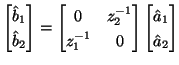$$\begin{bmatrix}\hat{b}_{1}\\ \hat{b}_{2}\\ \end{bmatrix}= \begin{... ...{-1}&0\\ \end{bmatrix} \begin{bmatrix}\hat{a}_{1}\\ \hat{a}_{2}\\ \end{bmatrix}$$ (4.121)

and shown in Figure 4.45(a) bears some resemblance to the lumped unit element discussed initially in §2.3.4; it is clearly lossless (because it merely implements a pair of shifts), but, unlike the unit element, it is no longer reciprocal. In this last respect, we remark that a multidimensional element so defined is perhaps closer in spirit to a generalization of the so-called quasi-reciprocal line (QUARL) proposed by Fettweis [46]. The two port resistances are assumed identical and equal to some positive constant $R$. When the spatial dependence is expanded out, it appears as an entire array of unit elements, as in Figure 4.45(b), where we have assumed

$$z_{1}^{-1} = z^{-\frac{1}{2}}w^{-\frac{1}{2}}\hspace{1.0in}z_{2}^{-1} = z^{-\frac{1}{2}}w^{\frac{1}{2}}$$

where $z^{-\frac{1}{2}}$ and $w^{-\frac{1}{2}}$ correspond, respectively, to unit shifts in time and space by $T/2$ and $\Delta/2$. We have thus chosen $T_{1} = T_{2} = \Delta/\sqrt{2}$.

Figure 4.45: (a) Multidimensional unit element at steady state making use of shifts in directions $t_{1}$ and $t_{2}$ and (b) its steady state schematic when spatial dependence is expanded out.

This element, like the standard unit element, is defined in the discrete (time and space) domain, and using wave variables. Rewriting the scattering relation in terms of steady-state discrete voltage and current amplitudes, (4.104) becomes the impedance relationship

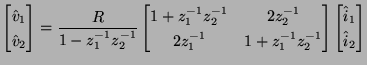$$\begin{bmatrix}\hat{v}_{1}\\ \hat{v}_{2}\\ \end{bmatrix}= \frac{R... ...2}^{-1}\\ \end{bmatrix}\begin{bmatrix}\hat{i}_{1}\\ \hat{i}_{2}\\ \end{bmatrix}$$ (4.122)