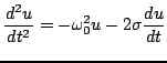
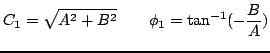
Damping intervenes in any musical system, and, in the simplest case, may be modelled through the addition of a ``linear loss" term to a given system. In the case of the simple harmonic oscillator, one may add damping as
| (3.62) |
 |
(3.63) |
 |
(3.64) |
| (3.66) |
 |
(3.67) |
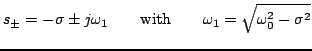
The case of large damping, i.e.,
![]() is of mainly academic interest in musical acoustics. The main point here is that for
is of mainly academic interest in musical acoustics. The main point here is that for
![]() , the solution will consist of two exponentially damped terms, and for
, the solution will consist of two exponentially damped terms, and for
![]() , degeneracy of the roots of the characteristic solution leads to some limited solution growth.
, degeneracy of the roots of the characteristic solution leads to some limited solution growth.
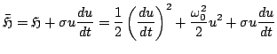
The energetic analysis of (3.61) is a simple extension of that for system (3.1). One now has, after again multiplying through by
![]() ,
,
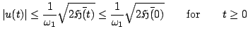
The bounds (3.68) and (3.70) obtained through frequency domain and energetic analysis, respectively, are distinct. Notice, in particular, that bound (3.70) is insensitive to the addition of loss, but, at the same time, is more general than bound (3.68), which requires the assumption of small damping (i.e.,
![]() ). It is possible to reconcile this difference by extending the energetic analysis somewhat in the following way.
). It is possible to reconcile this difference by extending the energetic analysis somewhat in the following way.
First, note that although
![]() will be monotonically decreasing in the case of linear loss, by (3.69), the specifics of its rate of decay are unclear. To this end, define the function
will be monotonically decreasing in the case of linear loss, by (3.69), the specifics of its rate of decay are unclear. To this end, define the function
![]() by
by
On the other hand,
![]() , in contrast to
, in contrast to
![]() , is not necessarily a non-negative function of the state
, is not necessarily a non-negative function of the state ![]() and
and ![]() . This non-negativity property is crucial in obtaining bounds such as (3.14). To this end, it is worth determining the conditions under which
. This non-negativity property is crucial in obtaining bounds such as (3.14). To this end, it is worth determining the conditions under which
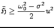
![]() is non-negative. First note that
is non-negative. First note that
 |
(3.73) |
 |
(3.74) |
 |
(3.75) |
In general, true energy functions such as
![]() for physical systems are non-negative, and the introduction of modified energetic quantities such as
for physical systems are non-negative, and the introduction of modified energetic quantities such as
![]() , for which non-negativity conditions must be determined, might seem to be a needless complication. On the other hand, for numerical approximations, as will be seen shortly, the discrete equivalent of the system energy is not necessarily non-negative, and the determination of non-negativity conditions leads to numerical stability conditions. Thus the simple analysis above serves as a useful example, in miniature, of what will follow in this book. Even in the discrete case, it will sometimes be useful to introduce modified energetic quantities such as
, for which non-negativity conditions must be determined, might seem to be a needless complication. On the other hand, for numerical approximations, as will be seen shortly, the discrete equivalent of the system energy is not necessarily non-negative, and the determination of non-negativity conditions leads to numerical stability conditions. Thus the simple analysis above serves as a useful example, in miniature, of what will follow in this book. Even in the discrete case, it will sometimes be useful to introduce modified energetic quantities such as
![]() , especially when dealing with certain types of non-centered finite difference schemes.
, especially when dealing with certain types of non-centered finite difference schemes.