Finite Difference Scheme

The damped oscillator (3.61) may be dealt with in a variety of ways. A simple scheme is the following:

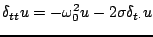$$\delta_{tt}u = -\omega_{0}^2 u-2\sigma\delta_{t\cdot}u$$ (3.76)

which, when the operator notation is expanded out, leads to the recursion

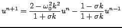$$u^{n+1}=\frac{2-\omega_{0}^2 k^2}{1+\sigma k}u^{n}-\frac{1-\sigma k}{1+\sigma k} u^{n-1}$$ (3.77)

This is again a recursion of temporal width three.

The characteristic equation will now be

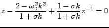$$z-\frac{2-\omega_{0}^2 k^2}{1+\sigma k}+\frac{1-\sigma k}{1+\sigma k}z^{-1}=0$$ (3.78)

The roots may be written explicitly as

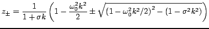$$z_{\pm} = \frac{1}{1+\sigma k}\left(1-\frac{\omega_{0}^2 k^2}{2}\pm\sqrt{\left(1-\omega_{0}^2 k^2/2\right)^2-(1-\sigma^2 k^2)}\right)$$ (3.79)

Though a direct analysis of the above expressions for the roots is possible, if one is interested in bounding the magnitudes of the roots by unity, it is much simpler to employ the conditions (2.11), which yield, simply,

$$k\leq \frac{2}{\omega_{0}}$$ (3.80)

In other words, the stability condition for scheme (3.76), which involves a centered difference approximation for the loss term, is unchanged from that of the undamped scheme (3.18). On the other hand, a more direct examination of the behaviour of the roots given above can be revealing; see Problem 3.6.

Energetic analysis also yields a similar condition. Multiplying (3.76) by $\delta_{t\cdot}u$ gives, instead of (3.36),

$$\delta_{t+}{\mathfrak{h}} = -2\sigma\left(\delta_{t\cdot}u\right)^2 \leq 0$$ (3.81)

where ${\mathfrak{h}}={\mathfrak{t}}+{\mathfrak{v}}$, with ${\mathfrak{t}}$ and ${\mathfrak{v}}$ defined as before in (3.37). From the previous analysis, it remains true that ${\mathfrak{h}}$ is non-negative under the condition (3.80), in which case one may deduce that

$${\mathfrak{h}}^{n} \leq {\mathfrak{h}}^{n-1} \leq {\mathfrak{h}}^{0}$$ (3.82)

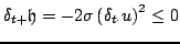
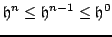
for all $n\geq 1$. In other words, the discrete energy function is monotonically decreasing. As the expression for the energy is the same as in the lossless case, one may again arrive at a bound on solution size, namely

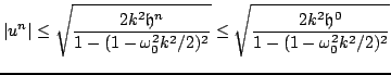$$\vert u^{n}\vert\leq \sqrt{\frac{2k^2{\mathfrak{h}}^n}{1-(1-\omeg... ...^2 k^2/2)^2}}\leq\sqrt{\frac{2k^2{\mathfrak{h}}^0}{1-(1-\omega_{0}^2 k^2/2)^2}}$$ (3.83)

The scheme above makes use of a centered difference approximation to the loss term. Consider the following non-centered scheme:

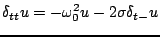$$\delta_{tt}u = -\omega_{0}^2 u-2\sigma\delta_{t-}u$$ (3.84)

The characteristic equation will now be

$$z-\left(2-\omega_{0}^2 k^2+2\sigma k\right)+\left(1-2\sigma k\right)z^{-1}=0$$ (3.85)

The condition (2.11) now gives the following condition on $k$ for numerical stability:

$$k\leq\frac{2}{\omega_{0}}\left(-\sigma +\sqrt{\sigma^2+\omega_{0}^2}\right)$$ (3.86)

See Problem 3.7.

This non-centered scheme is only first order accurate, but, if the loss parameter $\sigma$ is small, as it normally is for most systems in musical acoustics, the solution accuracy will not be severely degraded. Although in this case, one can arrive at an explicit update using centered or non-centered difference approximations, in the distributed setting, such backward difference approximations can be useful in avoiding implicit schemes, which are generally much more costly in terms of implementation.