


Next: As First-Order System
Up: The Simple Harmonic Oscillator
Previous: Sinusoidal Solution
Contents
Index
Energy
In is straightforward to derive an expression for the energy of the simple harmonic oscillator. Recalling the discussion at the beginning of Section 2.4.1, after multiplying (3.1) by
 , one arrives at
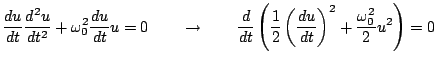 |
(3.8) |
Writing
 |
(3.9) |
with
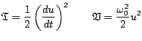 |
(3.10) |
one clearly has
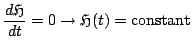 |
(3.11) |
When scaled by a constant with dimensions of mass,
 ,
,
 and
and
 are the kinetic energy, potential energy, and total energy (or Hamiltonian) for the simple harmonic oscillator.
In order to arrive at a bound on solution size in this case, one may first observe that
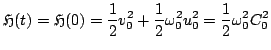 |
(3.12) |
where  is defined in (3.6). Then, noting the non-negativity of
and
, as defined in (3.10), one has
is defined in (3.6). Then, noting the non-negativity of
and
, as defined in (3.10), one has
 |
(3.13) |
and, using the form of
 , one has, finally,
 |
(3.14) |
which is the same as the bound obtained in the previous section. In this case, however, one has made no a priori assumptions about the form of the solution. A bound on  can clearly also be obtained; though not so useful for the SHO given the strength of the above condition on
  itself, such bounds do come in handy when dealing with distributed systems under free boundary conditions. See Problem 3.1.
This type of analysis, in which frequency domain analysis is avoided, has also been applied to the analysis of numerical simulation techniques, and is sometimes referred to as the energy method [171]. It is somewhat more general than frequency domain analysis in that it may be applied to nonlinear systems as well as linear ones. It is worth noting that even though it was stated at the beginning of this section that an energy would be ``derived" from system (3.1), one could equally well begin from the expressions for kinetic and potential energy given in (3.10), and, through the application of variational principles, arrive at (3.1). This variational point of view dominates in the finite element simulation community.
Next: As First-Order System
Up: The Simple Harmonic Oscillator
Previous: Sinusoidal Solution
Contents
Index
Stefan Bilbao
2006-11-15