Numerical Decay Time

Like frequency, loss is an extremely important perceptual characteristic of a musical system, in that it determines a characteristic decay time; as has been shown in the case of the SHO, frequency can be altered through numerical approximation, and, as one might expect, so can the decay time. It is thus worth spending a few moments here in determining just how much distortion will be introduced through finite difference approximations.

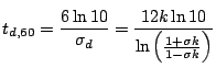
First consider the solution (3.65) to the SHO with loss, under normal (low-loss) conditions. Clearly the solution is damped by a decaying exponential, and the 60 dB decay time $t_{60}$ (in amplitude) may be defined as

$$t_{60} = \frac{6\ln 10}{\sigma}$$ (3.87)

Considering now the simple difference scheme (3.76), if the stability condition (3.80) is respected, and again under low-loss conditions, the roots $z_{\pm}$ of the characteristic polynomial (3.78) will be complex conjugates, of magnitude

$$\vert z\vert = e^{-\sigma_{d}k} = \sqrt{\frac{1-\sigma k}{1+\sigma k}}$$ (3.88)

Here, $\sigma$ is the loss parameter for the model system (3.61), and $\sigma_{d}$ is that corresponding to the finite difference scheme. One can then define a numerical 60 dB decay time $t_{d,60}$ by

$$t_{d,60} = \frac{6\ln 10}{\sigma_{d}} = \frac{12k\ln 10 }{\ln\left(\frac{1+\sigma k}{1-\sigma k}\right)}$$ (3.89)

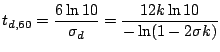
For scheme (3.84), for instance, which uses a non-centered approximation to the loss term, the magnitudes of the solutions to the characteristic polynomial (3.85) will be, again under low loss conditions,

$$\vert z\vert = e^{-\sigma_{d}k} = \sqrt{1-2\sigma k}$$ (3.90)

implying that

$$t_{d,60} = \frac{6\ln 10}{\sigma_{d}} = \frac{12k\ln 10 }{-\ln (1-2\sigma k)}$$ (3.91)

It is useful to plot the relative decay time $t_{d,60}/t_{60}$ for the schemes mentioned above-see Figure 3.4.

Figure 3.4: The relative 60 dB decay time $t_{d,60}/t_{60}$ for scheme (3.76), as a solid black line, and for scheme (3.84), as a dotted black line, plotted against $\sigma k$.

For scheme (3.76), the numerical decay time is closer than 99$\%$ of the true decay time for $\sigma k\leq 0.17$. For a sample rate of 44.1 kHz (implying $k = 1/44100$), this implies that for decay times greater than $t_{60}=0.0018$ s, the numerical decay time will not be noticeably different than that of the model system. For scheme (3.76), the 99$\%$ threshold is met for $t_{60}\geq 0.031$ s. These decay times are quite short by musical standards, and so it may be concluded that numerical distortion of decay time is not of major perceptual relevance, at least at reasonably high sample rates.

Although in the two examples of numerical schemes above, the numerical decay time is independent of $\omega _{0}$ (as it is for the model system), this is not necessarily always the case. See Problem 3.8.